BIOL 497/597 - Genomics & Bioinformatics
Chapters
Sven Buerki - Boise State University
2026-01-30
1 Introduction
This webpage contains materials associated with the chapters covered in BIOL 497/597 – Genomics & Bioinformatics, a course taught at BSU. In addition to this content, the instructor provides PDF presentations and hands-on tutorials designed to support in-class exercises (see, for example, Chapter 4).
3 Chapter 1
3.1 Goal
The goal of this chapter is to establish the foundational genomics concepts required for the remainder of the course.
Students will develop a shared theoretical framework—including key definitions (see Lexicon)—that underpins genome sequencing, assembly, and annotation workflows.
In this chapter, an emphasis will be placed on the structure, organization, and function of DNA and RNA as they directly inform the design and interpretation of genomic research projects.
3.2 Chapter Structure
The learning outcomes of this chapter will be addressed through a combination of a lecture, which introduces core genomics concepts and definitions, and an in-class group activity focused on exploring genome diversity and variation in assembly completeness.
3.3 Learning Outcomes
The key learning outcomes of this chapter are:
- Understand the differences between genetics and genomics.
- Genetics focuses on individual genes and how traits are inherited, emphasizing heredity. In contrast, genomics examines the entire genome (all genes), their interactions with each other and with the environment, and how these interactions influence phenotype. Genomics therefore provides a broader perspective and relies heavily on advanced technologies for large-scale data analysis. An analogy is that genetics is like reading individual words, whereas genomics is like reading the entire book in its full context.
- Understand the central dogma: DNA is transcribed into RNA, which is translated into protein.
- This will be especially important for the Lab. report.
- Appreciate the diversity of genome organization in organelles, prokaryotes, and eukaryotes (e.g., Saitou, 2013).
- Understand how organelle genomes have contributed to the evolution of eukaryotic chromosomes and how this impacts genome assembly project design (e.g., Timmis et al., 2004).
- Appreciate that eukaryotic genomes contain extensive and diverse repetitive regions (e.g., the sagebrush genome contains approximately 78% repetitive elements, Melton et al., 2022).
- Appreciate the diversity of published genomes and variation in their levels of completeness.
- This topic will be further investigated in a group activity
- Understand the importance of computer science and bioinformatics in generating raw sequencing data and assembling genomes.
- Understand the major challenges associated with sequencing and assembling genomes.
3.4 Resources
This chapter is mostly based on the following resources:
- Aransay (2016) - Sequencing strategy
- Asaf et al. (2016) - Synonymous vs. non-synonymous substitutions
- Bradnam et al. (2013) - De novo genome assembly contest
- Doležel et al. (2007) - Flow cytometry
- Ellestad et al. (2022) - SNPs in Vanilla
- Greenberg and Soreq (2013) - Alternative splicing
- Hu et al. (2021) - SNPs in Corn
- Liao et al. (2023) - Repeats in human genome
- Melton et al. (2021) - Paralogs in sagebrush
- Melton et al. (2022) - Sagebrush genome and repeats
- Nurk et al. (2022) - The complete sequence of a human genome
- Öhman and Bass (2001) - RNA editing
- Pellicer et al. (2010) - Plant genome size
- Rice et al. (2013) - Plant mitochondrial genome evolution
- Sen et al. (2011) - Chloroplast genome function and evolution
- Timmis et al. (2004) - Evolution of chloroplast genomes (gene trafficking)
3.5 Lecture
The presentation associated with this class is available here:
3.6 🤝 Group Activity: Exploring Genome Diversity and Completeness
3.6.1 Learning Outcome
Students appreciate the diversity of published genomes and the variation in their levels of completeness by exploring and comparing genome assemblies available in the NCBI database.
3.6.2 Activity Overview
In this 1 hour and 40 minutes in-class group activity, students work in small groups to explore, compare, and critically evaluate genome assemblies from different organisms using NCBI resources.
The objective is to recognize how genome completeness varies across taxa and sequencing strategies, and to reflect on the biological and technical factors that influence genome assembly quality.
3.6.3 Materials
- NCBI – National Center for Biotechnology Information
- NCBI – Genome Database
- Lexicon
- Lecture Material (from slide 56 onward)
3.6.4 Activity Structure (1 hour 40 minutes)
3.6.4.1 Context and Setup (15 minutes)
As discussed in lecture:
- Published genomes vary widely in their level of completeness and overall quality.
- Genome assembly quality is influenced by biological features (e.g., genome size, repetitive content, ploidy) as well as technical factors (e.g., sequencing technology, sequencing depth).
- The goal of this activity is to critically evaluate real genomic data rather than to label genomes as “good” or “bad.”
During this time, key assembly metrics (e.g., assembly level, N50, scaffold vs. contig) are reviewed, and students clarify expectations and terminology before group work begins.
3.6.4.2 Group Exploration (35 minutes)
Students will work in groups of 3–4. Each group should include at least one graduate student to help guide the discussion.
Each group selects two organisms representing different biological categories (e.g., model vs. non-model organisms, prokaryotes vs. eukaryotes).
Suggested organism pairings include:
- Homo sapiens vs. Artemisia tridentata
- Arabidopsis thaliana vs. a non-model plant species
- Escherichia coli vs. a eukaryotic genome
For each organism, groups navigate to the NCBI Genome page and record the following information:
- Assembly level (Complete Genome, Chromosome, Scaffold, or Contig)
- Genome size
- Number of scaffolds or contigs
- N50 value (if available)
- Sequencing technology (if reported)
- Year of release
- Annotation status (e.g., RefSeq, GenBank only)
Groups are encouraged to explore multiple assemblies for the same organism (when available) to observe how assembly quality has changed over time.
💡 Information
- Use this activity to become familiar with genomics terminology by consulting the Lexicon and other reliable resources as needed.
Throughout this phase, questions, comparisons, and observations naturally emerge within and across groups.
3.6.4.3 Group Discussion and Synthesis (30 minutes)
Within each group, students discuss the following questions:
- How do the two genomes differ in terms of size, completeness, and assembly quality?
- Consider metrics or features that indicate completeness, such as the number of scaffolds/contigs, N50, and presence of core genes.
- Consider metrics or features that indicate completeness, such as the number of scaffolds/contigs, N50, and presence of core genes.
- What biological factors (e.g., genome size, repetitive content, ploidy) might explain differences in genome completeness or assembly quality?
- What technical, historical, or funding-related factors (e.g., sequencing technology, coverage, date of publication) might explain these differences?
- Which genome would you trust more for downstream analyses, and why?
- Identify the evidence supporting your choice.
- Identify the evidence supporting your choice.
- How might your criteria for evaluating genome completeness influence the biological conclusions you could draw from these assemblies?
💡 Tip: Focus on evidence from assembly metrics and consider both biological and technical contexts. Use this discussion to practice critical evaluation of genomic data.
Each group identifies two key observations they find most informative or surprising and prepares to share them with the class.
3.6.4.4 Whole-Class Debrief (20 minutes)
Groups share their key observations with the class.
As a class, students collectively highlight and discuss:
- Common patterns observed across taxa,
- Differences between model and non-model organisms,
- The impact of sequencing technology and assembly strategy on genome completeness,
- Questions or concerns that arise when evaluating genome quality for downstream analyses.
Key points raised by the class are recorded and revisited in later chapters on genome assembly and annotation, reinforcing how early evaluation of genome quality shapes genomic research decisions.
4 Chapter 2
4.1 Goal
The goal of this chapter is to provide students with a conceptual understanding of next-generation sequencing (NGS) technologies, including their underlying principles and practical applications. Students will apply this knowledge by independently researching a sequencing platform and synthesizing their findings in an individual mini-report (see Mini-Report 1).
4.2 Chapter Structure
The learning outcomes of this chapter are addressed through a combination of a lecture, which introduces next-generation sequencing technologies, and a group activity that develops genomics terminology and critical reading skills by analyzing a publication on the giant panda genome. Finally, the lecture will also provide key concepts for Mini-Report 1.
4.3 Learning Outcomes
- Learn the terminology associated with next-generation sequencing (NGS) that underpins genome assembly and annotation (see Lexicon).
- Understand the general principles of genome sequencing (wet-lab) and genome assembly (bioinformatics workflows).
- Be familiar with the major NGS platforms and their limitations (see Mini-Report 1):
- Illumina
- PacBio
- Oxford Nanopore
- Illumina
- Become proficient in handling NGS data outputs, particularly FASTA and FASTQ files.
- Learn how to assess nucleotide quality using Phred quality scores.
- Become familiar with reading the genomics literature (see Group Activity).
4.4 Resources
4.4.1 Publications
This chapter is mostly based on the following resources:
- Heather and Chain (2016) - The sequence of sequencers: The history of sequencing DNA
- Ignatov (2019) - Fragmenting DNA for NGS sequencing
- Li, Fan, et al. (2009) - Giant Panda genome paper
- Marx (2023) - Long-read sequencing
- Nurk et al. (2022) - The complete sequence of a human genome
- Satam et al. (2023) - Next-Generation Sequencing technology: current trends and advancements
- Watson and Crick (1953) - Structure for Deoxyribose Nucleic Acid
💡 Note
- These publications will be very helpful to complete Mini-Report 1.
4.4.2 Web Resources
The following resources are helpful to complete Mini-Report 1 and support reading scientific publications (Journal Club):
- BSU Sequencing Core. Our University is offering a suite of genomics services and they have an Illumina NextSeq 1000 instrument.
- Overview of Next-Generation Sequencing technologies
- Phred quality score
- The Human Genome Project
- How to read a scientific paper
- How to (seriously) read a scientific paper
4.5 Lecture
The presentation associated with this class is available here:
4.6 🤝 Group Activity: Reading the Giant Panda Genome Paper
4.6.1 Paper
- Li, Fan, et al. (2009) – Giant Panda genome paper
- Nature 463: 311–317. DOI: 10.1038/nature08696
- Nature 463: 311–317. DOI: 10.1038/nature08696
- Available on Google Drive
4.6.2 Learning Outcome
Students develop skills in reading and critically evaluating genomics publications by analyzing a real genome assembly study.
4.6.3 Activity Overview
In this 1 hour and 40 minutes in-class activity, students work in groups of 3–4 to explore the giant panda genome paper (each group includes at least one graduate student to help guide the discussion).
The goals are to:
- Interpret genome assembly metrics
- Evaluate technical and biological conclusions
- Connect genomic data to scientific reasoning
- Practice evidence-based discussion and group synthesis
4.6.4 Materials
- Full text of the giant panda genome paper
- How to read a scientific paper
- How to (seriously) read a scientific paper
- Instructor presentation summarizing the publication and initiating discussion: Journal Club: Giant Panda
- NCBI Genome Database (optional reference)
- Lexicon
4.6.5 Activity Structure (1 hour 40 minutes)
4.6.5.1 Context and Setup (15 minutes)
- Review key assembly metrics introduced in Chapter 1’s group activity and in slides 8–10 of this presentation (e.g., scaffolds, N50, assembly completeness).
- Discuss the importance of evaluating both technical methods and biological conclusions when reading genomics papers.
- Clarify expectations for group work, including collaborative note-taking and critical discussion.
4.6.5.2 Group Reading and Annotation (30 minutes)
- Groups read the paper, focusing on methods, results, and figures.
- Annotate the text or take notes on terms, methods, metrics, or claims that are unclear.
- Use the Lexicon to clarify unfamiliar genomics terminology (e.g., N50, scaffolds, assembly completeness).
- Identify sections where assembly methods influence biological interpretations.
4.6.5.3 Guided Group Questions (30 minutes)
Each group collaboratively answers the following questions:
- Research Motivation: What biological or evolutionary questions drive this genome project? Why is it significant?
- Sequencing Strategy: Which sequencing technologies are used? What limitations or biases might they introduce?
- Assembly Quality: How do the authors evaluate assembly completeness and quality? Which metrics are most informative?
- Biological Insights: What conclusions do the authors draw (e.g., diet, metabolism, evolution)? How strong is the evidence?
- Historical Context and Impact: When was this paper published, and why was it considered groundbreaking at the time? How did assembling a eukaryotic genome using only Illumina data influence subsequent genome projects and the development of modern genomics?
- Reproducibility and Critique: What information allows others to reproduce the study? How could modern sequencing technologies and assembly approaches improve this work today?
Tip: Assign one or two questions to each group member to analyze in depth, then share answers within the group to build consensus.
4.6.5.4 Group Synthesis and Preparation for Class Discussion (15 minutes)
- Each group identifies two to three key insights or critical questions they want to share with the class.
- Groups designate one or two group members to serve as spokespersons for the whole-class debrief and discussion.
- Prepare a short summary (bullet points or figure highlights) to support discussion.
- Focus on evidence-based reasoning and on how assembly metrics relate to biological conclusions.
4.6.5.5 Whole-Class Debrief and Discussion (20 minutes)
- Groups present their key insights or critical questions to the class.
- Class collectively identifies:
- Patterns in assembly quality and completeness
- Connections between technical methods and biological conclusions
- Strengths and limitations of the study
- Lessons for reading and evaluating genomics publications
- Patterns in assembly quality and completeness
💡 Tip: Treat figures and tables as primary evidence. Focus on interpreting data rather than relying on narrative text. Discuss observations collaboratively, highlighting multiple perspectives.
4.7 🧠 Quiz: Planning a Eukaryotic Genome Assembly
4.7.1 Objective
This quiz asks you to think about the essential biological information needed before starting a de novo genome assembly project for a eukaryotic organism.
4.7.2 👥 How This Quiz Works
- Students work in groups of 3–4.
- The quiz has two group-work parts (15 minutes each) followed by a whole-class debrief (10 minutes).
- Groups should agree on shared answers and be prepared to explain their reasoning.
- Not every group needs to answer every question aloud — the goal is to compare ideas and build a shared understanding as a class.
Focus on reasoning, not just short answers.
4.7.3 Part 1 — Key Biological Information (15 minutes)
Before beginning a genome assembly project, researchers must understand fundamental properties of the genome they want to sequence.
Question 1
What are the two most important pieces of biological information you would want to know before starting a de novo genome assembly project for a eukaryotic organism?
✏️ Write your answer in 1–2 sentences.
Question 2
Why is each of these two pieces of information important for genome assembly?
Describe how they influence sequencing strategy, assembly difficulty, or downstream analysis.
✏️ Write 2–4 sentences.
4.7.4 Part 2 — How Could You Obtain This Information? (15 minutes)
Now think about how scientists would measure or estimate the types of genome features you identified in Part 1.
For each of the biological properties your group selected, answer the following:
Question 3
What experimental approaches could be used to measure or estimate this property before or during a genome sequencing project?
Consider lab-based techniques, microscopy, or molecular methods.
Question 4
What sequence-based or computational approaches might help estimate this property once some sequencing data become available?
✏️ For each property, list at least one experimental and one computational approach, and briefly describe what information each method provides.
4.7.5 Part 3 — Whole-Class Debrief (10 minutes)
- Groups volunteer to share their answers and reasoning.
- The class compares different approaches and discusses:
- Why are these two pieces of biological information foundational for assembly design
- How different methods provide complementary information
- What additional genome features might complicate assembly
- Why are these two pieces of biological information foundational for assembly design
The goal of this discussion is to connect biological knowledge with practical genome assembly planning.
4.8 Mini-Report 1
As part of this chapter, students are tasked to to produce individual mini-reports on the following sequencing platforms and their associated technologies:
- Sequencing platform 1: Illumina.
- Sequencing platform 2: PacBio.
- Sequencing platform 3: Oxford Nanopore.
More details on this assignment is available here.
💡 Disclaimer
- Warning: For this assignment, students are not allowed to use AI to complete their work.
- Questions or concerns: If you need assistance, please contact the instructor at svenbuerki@boisestate.edu.
5 Chapter 3
5.1 Goal
The goal of this chapter is to help you understand how biological data are stored, organized, and accessed in modern genomics.
By the end of the chapter, you should feel confident navigating major molecular databases and understanding how they support de novo genome assembly, annotation, and downstream biological interpretation.
5.2 Chapter Structure
The learning outcomes of this chapter are addressed through a combination of:
- A lecture, which introduces molecular databases and their role in genomics
- A mandatory assignment, Mini-Report 2, which allows you to explore different types of molecular databases and understand how they contribute to de novo genome assembly and annotation
Together, these components will help you connect theoretical knowledge about databases with practical skills in retrieving and using genomic data.
5.3 Learning Outcomes
By the end of this chapter, you will be able to:
- Explain the role of computer science and bioinformatics in modern molecular biology, including how they support:
- The production of raw biological data
- The creation and maintenance of molecular databases
- The archiving and curation of biological data
- The distribution of data via the internet
- The development of information-retrieval tools for biological research
- The production of raw biological data
- Describe the purpose, structure, and content of major molecular biology databases that are essential for genome assembly and annotation, including:
- Nucleic acid sequence databases
- Protein sequence databases
- Gene Ontology databases
- Metabolic pathway databases
- Specialized, annotated genome portals
- Nucleic acid sequence databases
- Apply basic bioinformatics protocols to query genomic information and remotely download sequence data from GenBank
- (These practical skills will be further developed in Mini-Report 3 and Chapter 4.)
5.4 Resources
5.4.1 Publications
This chapter is primarily based on the following resources:
5.4.2 Web Resources
- International Nucleotide Sequence Database Collaboration (INSDC)
- NCBI — National Center for Biotechnology Information
- NCBI BioProject Help Book: This guide provides definitions of terms associated with data submissions to NCBI.
5.5 Lecture
The presentation associated with this class is available here:
5.6 Data Availability
To support reproducibility and transparency in science, research institutions, funding agencies, and journals increasingly require that researchers make their data publicly accessible. This typically involves:
- Submitting genomic and other molecular data to accredited public repositories (such as NCBI) where the data can be freely accessed and reused
- Including a data availability statement in publications that clearly explains where and how the data can be accessed
To better understand these practices, review:
- An example of a journal data policy from the journal G3
- A real data availability statement from the sagebrush genome study (Melton et al., 2022)
These examples illustrate how researchers communicate where their data are stored and how other scientists can access them.
5.7 Exercises
The goal of these exercises is to help you become familiar with NCBI databases and understand how genomic data are linked to scientific publications.
5.7.1 1. Explore NCBI
Go to NCBI and spend a few minutes exploring its structure.
Identify the main types of databases available (e.g., Nucleotide, Genome, SRA, BioProject, Taxonomy).
5.7.2 2. Investigating the Sagebrush Genome Project
Using the paper by Melton et al. (2022) and NCBI resources, answer the following questions about the sagebrush (Artemisia tridentata; family Asteraceae) genome project:
- What is the BioProject accession number?
- How many SRA experiments were generated?
- What type(s) of sequencing technology were used to produce the SRA data?
- How much sequencing data was generated (in Gbases and terabytes)?
- What is the assembly level of the genome?
- What is the reported genome size (in Gb)?
- What is the estimated genome coverage?
- What assembly method or software was used?
5.7.3 3. Comparing Genomes in the Giant Panda
Using Li, Fan, et al. (2009) and NCBI:
- How many genome assemblies are currently available for the giant panda?
- In what ways do these assemblies differ (e.g., assembly level, sequencing technology, date of release)?
5.7.4 4. Your Organism of Interest
Search for your favorite organism in the NCBI Taxonomy database and explore its genomic resources.
- What types of genomic data are available (e.g., genome assembly, transcriptome, raw reads)?
- Is a reference genome assembly available? If so, at what assembly level?
Be prepared to briefly share what you found.
5.8 Mini-Report 2 – Molecular biology databases
To have a full overview of available molecular biology databases and assess their contributions to genome annotation, students are tasked to produce individual mini-reports on the following molecular databases:
- Molecular database 1: Protein sequences databases (e.g., Consortium, 2014).
- Molecular database 2: Gene ontology databases (e.g., Consortium, 2020).
- Molecular database 3: Metabolic pathways databases (e.g., Kanehisa et al., 2022).
More details on this assignment is available here.
6 Chapter 4
6.1 Bioinformatics Toolkit for Genomics
Before getting into conducting bioinformatics analyses to de novo assemble a draft nuclear genome, we will devote time to learn computing procedures. Please click here to access this material.
6.2 Aim and objectives
In this chapter, we aim at training students in producing a draft nuclear genome for a non-model organism using Illumina data.
The whole-genome shotgun (WGS) sequencing dataset published by Zhang et al. (2017) on the orchid species Apostasia shenzhenica is used as case-study. This dataset provides an opportunity to gain firsthand experience in analyzing NGS data. Zhang et al. (2017) have also produced RNA-Seq data, which were used in their study to support genome annotation. Zhang et al. (2017) is available in our shared Google Drive.
The chapter is subdivided into three parts:
- PART 1: Preparing/cleaning Illumina reads for de novo nuclear genome assembly and inferring genome size and complexity.
- PART 2: De novo genome assembly.
- PART 3: Validation of the draft genome.
Before you start working on Chapter 4, please make sure that you have completed the tutorials available here.
6.3 Download presentations
The two presentations (in pdf format) associated to material presented in Chapter 4 can be downloaded here:
6.4 Presenting the NGS data
Details on the WGS PE Illumina library studied here are provided in Figure 6.1. The SRA accession number is SRR5759389 and the most important information to know about this data are that the fragments insert-size of the library is 180 bp and that the length of each PE read is 90 bp. Note that the authors have performed a round of PCR amplification during their library preparation. This step is know to potentially introduce errors in reads, which could be identified by performing k-mer analyses.
The number of bases shown in Figure 6.1 was inferred as follows: \(\text{N bases} = \text{N. spots * reads length (bp)}\). In this example, \(\text{N bases} = 84.1e6 * 180 (90 + 90) = 15.1e9bp = 15.1Gbp\).
You can also obtain a rough estimate of haploid genome coverage (x) by using the following equation: \(\text{Raw haploid genome coverage (x)} = \text{N bases / Genome size (haploid)}\). In this example, \(\text{Raw haploid genome coverage (x)} = 15.1e9 / 471.0e6 = 32x\). The estimation of haploid genome size was taken from Zhang et al. (2017).
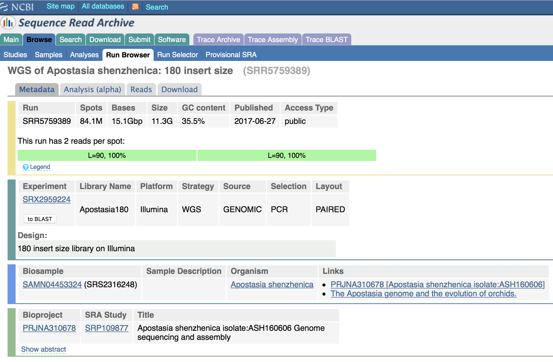
Figure 6.1: Details on the WGS library (SRA accession number: SRR5759389) used in this tutorial.
6.5 Write your own scripts
As you go along this document and perform analyses, please COPY ALL COMMAND LINES into an .Rmd document saved in a folder entitled Report/ (create this folder in your working directory; see below). Remember to comment your script (using #s). This will greatly help you in repeating your analyses or using parts of your code to create new scripts. Enjoy scripting!
6.6 Files location
Files for this chapter are deposited on each group Linux computer under the following path, which is shared between all the users on the computer: /home/Genomics_shared/Chapter_04/.
There are three folders in this project:
01_SRA/: This folder contains theSRAfile (SRR5759389_pe12.fastq) downloaded from theSRAdatabase. This file is very large, >35GB!02_Kmers_analyses/: This folder contains the structure that will be used for this tutorial. Each student will have to copy this folder onto the account prior to starting the analyses.03_Output_files/: This folder contains all the outputs files. Students can look at these files to help solve potential coding issues.
6.7 Software (incl. connecting off campus)
To support remotely connecting to the Linux computers and retrieving files (from the Linux computer to your personal computer), please make sure that you have installed the following software on your personal computer before pursing with this tutorial:
- Putty: This software will be required to remotely connect to the Linux computers if you have a Windows OS.
- FileZilla: This software will be useful to exchange files from the Linux computer to your personal computer.
If you are working from outside of the University network (= off campus) on your personal computer (e.g., you are not connect to the eduroam WiFi), then you will need to use the BSU VPN (Virtual Private Network) to connect to the BSU secured network prior to remotely connecting to your Linux computer account (using ssh protocol as taught in class; see Tutorials).
The BSU VPN software and instructions are available at this URL: https://www.boisestate.edu/oit-network/vpn-services/
6.8 PART 1: QCs, read cleaning and genome size
6.8.1 Analytical workflow
The overarching objective of this tutorial is to gain theoretical and bioinformatics knowledge on the steps required to prepare PE Illumina reads for de novo nuclear genome assembly as well as infer genome size and complexity (see Figure 6.2).
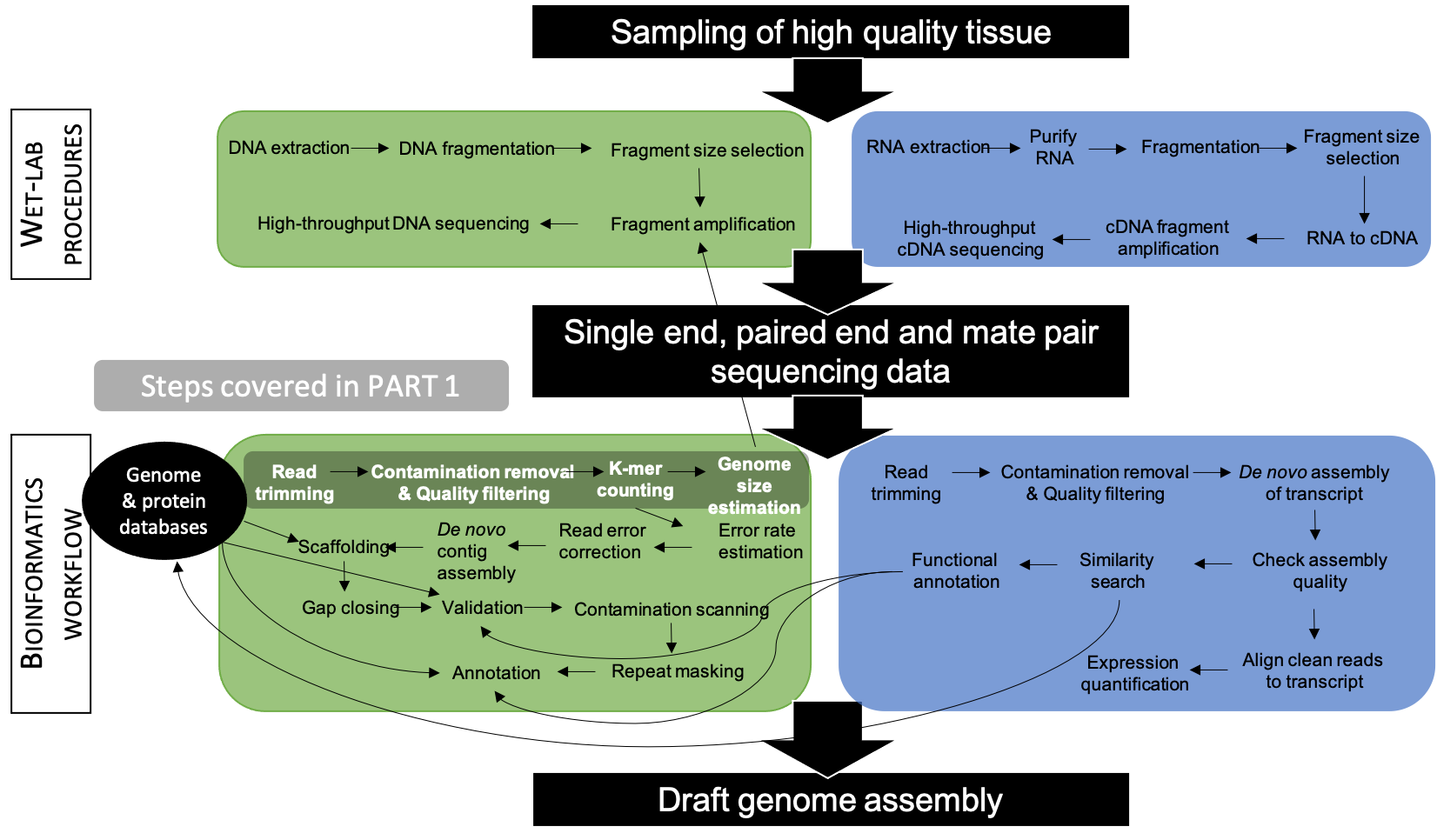
Figure 6.2: Workflow applied to assemble and annotate a genome for non-model organisms. Steps associated to PART 1 are highlighted in grey.
The five main steps associated to the objectives of PART 1 are as follows (see Figure 6.3):
- Step 1: Download SRA file containing raw WGS data and simultaneously convert it into an interleaved PE
fasqtformat file. This latter format (where both reads are paired and combined into one file) is the input for most bioinformatic programs. - Step 2: Infer reads Quality Checks (QCs) using standard statistics implemented in
FastQC(Andrews, 2012). - Step 3: Perform reads cleaning based on Phread scores and k-mer frequencies.
- Step 4: What’s “in” the reads? This will be done in two phases as follows:
- Infer and plot clean reads GC contents to assess potential contamination patterns.
- Map clean reads against reference genomes to assess the proportions of reads belonging to either nuclear or chloroplast genomes.
- Step 5: Estimate genome size and complexity (especially looking at repetitive elements and heterozygosity rate) using k-mer frequencies.
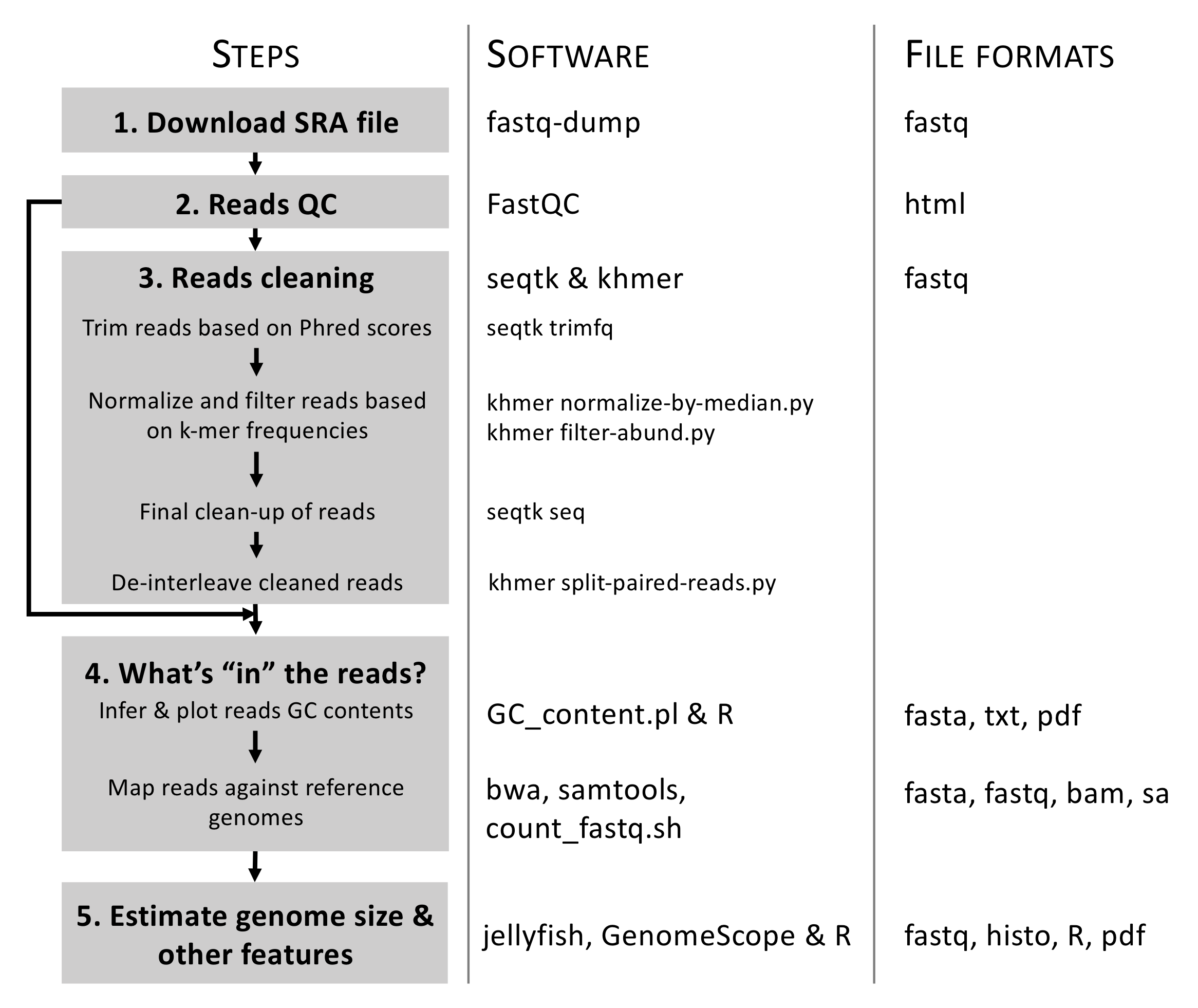
Figure 6.3: Overview of the analytical workflow applied here to prepare/clean Illumina reads for genome assembly and inferring genome size and complexity. Details on associated bioinformatic tools (here software) and file formats are also provided.
6.8.2 Copy the Project to your account
Before starting coding, each student has to copy the 02_Kmers_analyses/ folder project located in /home/Genomics_shared/Chapter_04 in their ~/Documents/ folder.
To do that, please execute the following commands in a Terminal window:
Remotely connect to your computer account using
sshStart a new
tmuxsession and rename itPart1Execute the code below to copy the data on your account:
#Navigate to /home/Genomics_shared/Chapter_04
cd /home/Genomics_shared/Chapter_04

#Copy all files in 02_Kmers_analyses/ in ~/Documents/ (This takes ca. 10 minutes to complete)
cp -r 02_Kmers_analyses/ ~/Documents/

#Navigate to ~/Documents/02_Kmers_analyses/ to start the analyses
cd ~/Documents/02_Kmers_analyses/
6.8.2.1 Questions
Use this resource to:
Which command can be applied to list the content of
02_Kmers_analyses/?
What is in
02_Kmers_analyses/?
How much space this folder takes on your computer?
6.8.3 Bioinformatic tools
Although all the bioinformatic tools (software) necessary to complete this tutorial are already installed on your Linux computers, URLs to their repositories (incl. documentations) are provided below together with details on their publications (when available). Software are sorted by steps in our analytical workflow (see Figure 6.3):
- Step 1:
fastq-dump: https://www.ncbi.nlm.nih.gov/sra/docs/toolkitsoft/. - Step 2:
FastQC(Andrews, 2012): https://www.bioinformatics.babraham.ac.uk/projects/fastqc/. - Step 3:
seqtk: https://github.com/lh3/seqtk.khmer(Crusoe et al., 2015): https://github.com/dib-lab/khmer.
- Step 4:
- Step 5:
jellyfish(Marçais and Kingsford, 2011): http://www.genome.umd.edu/jellyfish.html.GenomeScope(Vurture et al., 2017): http://qb.cshl.edu/genomescope/.
If you are remotely connecting to the Linux computers please install FileZilla to support file transfer. Please see section 6.8.6.2 for more details on how to set up remote connection for transferring files. Finally, the R software is also used in steps 4 and 5. You can find more details on this software in the Syllabus and Mini-Report webpages.
6.8.4 Step 1: Download SRA file
The SRA format (containing raw NGS data) can be quite difficult to play with. Here, we aim at downloading the WGS data, split PE reads, but store both reads (R1 and R2) in the same file using the interleaved format (Figure 6.3). This format is very convenient and is the entry point for most reads cleaning programs. This task can be done by using fastq-dump from the SRA Toolkit.
!!! DON’T EXECUTE THIS CODE !!!
The command to download the SRA file is available below, but please don’t execute the command since the file weighs >35GB and it takes a LONG time to download.
#Download PE reads (properly edited) in interleave format using SRA Toolkit
# !! DON'T EXECUTE THIS COMMAND !!
fastq-dump --split-files --defline-seq '@$ac.$si.$sg/$ri' --defline-qual '+' -Z SRR5759389  > SRR5759389_pe12.fastq
6.8.4.1 Questions
Open a Terminal, connect to your Part1 tmux session and navigate to the /home/Genomics_shared/Chapter_04/01_SRA folder using the cd command. This folder contains the SRA file (SRR5759389_pe12.fastq) that we will be using in this tutorial.
Use this resource to:
Identify a command to show the first 10 lines of
SRR5759389_pe12.fastq
What is the format of
SRR5759389_pe12.fastqand why do you reach this conclusion?
6.8.5 Step 2: Reads QCs
6.8.5.1 Theoretical background
To determine the quality of the raw Illumina data, we are conducting analyses to evaluate the following criteria:
- Basic Statistics
- Total # of sequences
- Sequence length
- %GC
- Per base sequence quality
- Quality scores across all bases
- Per sequence quality scores
- Quality score distribution across all sequences
- Per base sequence content
- Sequence content across all bases
- Per sequence GC content
- GC distribution over all sequences
- Per base N content
- N content across all bases
- Sequence Length Distribution
- Distribution of sequence lengths over all sequences
- Sequence Duplication Levels
- Percent of sequences remaining if deduplicated 70.44%
- Overrepresented sequences
- No overrepresented sequences
- Adapter Content
- Percent adapter
By intersecting results provided by these analyses, we can determine best-practices to conduct reads cleaning (incl. removal of contaminants) and determine whether our Illumina data are suitable for genomic analyses.
6.8.5.2 Bioinformatics
The program FastQC is used to obtain preliminary information about the raw Illumina data (see Figure 6.1). To perform this analysis do the following:
- Attach to your Part1
tmuxsession - Navigate to
~/Documents/02_Kmers_analyses/FastQCusingcd - Type to following command:
- Input:
01_SRA/SRR5759389_pe12.fastq - Output:
SRR5759389_pe12_fastqc.html
#Reads QCs with FastQC
./FastQC_program/fastqc -o ~/Documents/02_Kmers_analyses/FastQC/ /home/Genomics_shared/Chapter_04/01_SRA/SRR5759389_pe12.fastq
This step will have to be repeated after completion of the step3 (reads cleaning) to confirm that our reads trimming and cleaning procedure was successful. To inspect SRR5759389_pe12_fastqc.html click here.
6.8.5.3 Question
In small groups, inspect the output file and answer the following question:
What conclusions can you draw on the quality of the raw data based on the FastQC analysis?
Note: Go over each category outputted by the FastQC analyses and determine why these metrics were inferred and how they help you drawing conclusions on your data.
6.8.6 File transferring
At this stage, you will need to transfer SRR5759389_pe12_fastqc.html on your local computer to be able to inspect the results. This can be done using i) the scp protocol (but it only works on Unix-based operating systems) or ii) the sftp protocol as implemented in FileZilla (this works on all operating systems).
6.8.6.1 scp protocol
WARNING: This protocol works only on UNIX OS (Mac, Linux).
You can use the scp (Secure Copy Protocol) command to copy SRR5759389_pe12_fastqc.html or any other file to your local computer. This can be done as follows:
Open a
Terminalwindow on your computer and navigate (usingcd) where you want to store the target file.Type this command line:
#General syntax
scp USER@IP:PATH_ON_REMOTE_COMPUTER PATH_ON_YOUR_COMPUTER

#Example:
# To copy SRR5759389_pe12_fastqc.html on my computer from bio_11 user do:
scp bio_11@132.178.142.214:~/Documents/02_Kmers_analyses/FastQC/SRR5759389_pe12_fastqc.html .
6.8.6.2 sftp protocol
sftp is a SSH File Transfer Protocol that can be used to support file exchange between remote computers and your personal computer. This protocol is implemented in FileZilla and other free software.
To copy the output of the FastQC analysis on your computer do the following:
Open FileZilla on your personal computer and establish remote connection with Linux computer as shown in Figure 6.4. Once the connection is established:
- Navigate where the target file (
SRR5759389_pe12_fastqc.html) is located on the remote computer and select it. - Identify where the target file needs to be saved on your personal computer.
- Copy the file on your personal computer by dragging the target file from the remote to the local location.
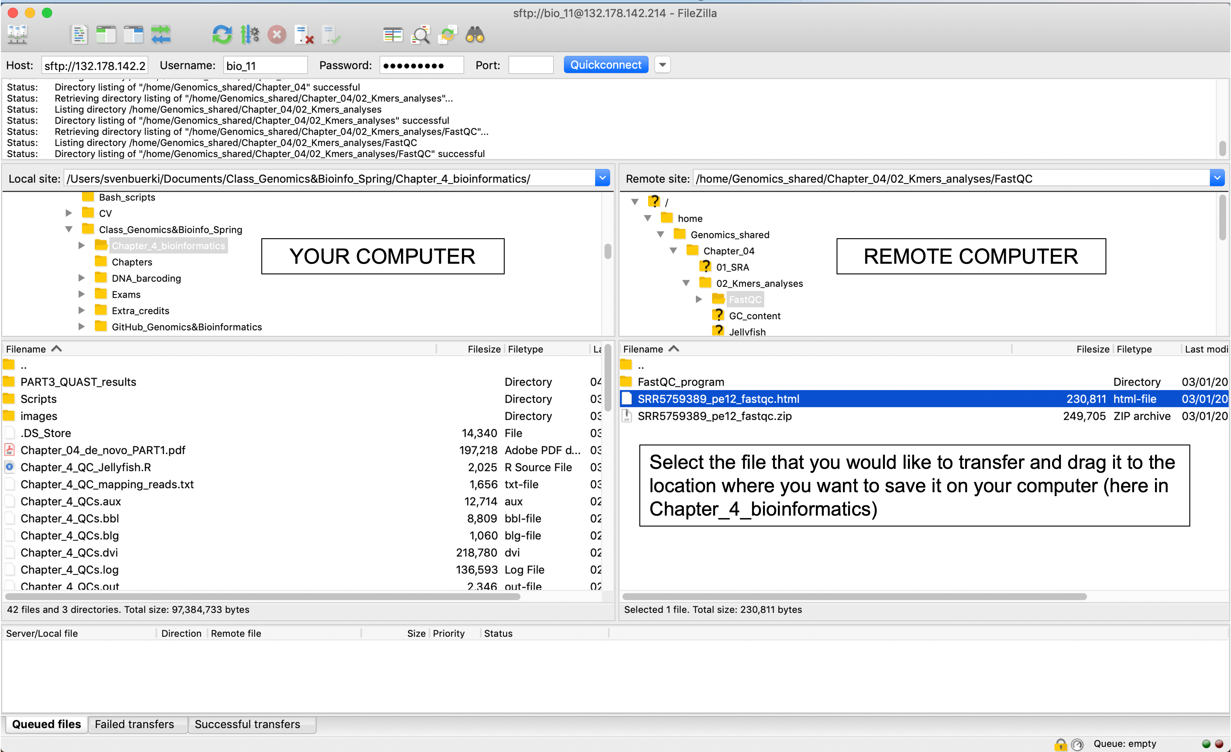
Figure 6.4: Snapshot of FileZilla program used to transfer files between computers.
This protocol will have to be replicated at different stages of this tutorial.
6.8.7 Step 3: Reads cleaning
This step is at the core of our analytical workflow. It is paramount to conduct thorough reads cleaning when assembling a nuclear genome due to the very nature of this genome (i.e. repetitive elements, heterozygosity, recombination, etc…). In this case, aim at minimizing the effect of PCR errors, which could jeopardize our assembly by creating false polymorphism. In addition, de novo genome assembly is computing intensive and by properly cleaning reads we will dramatically decrease RAM requirements.
6.8.7.1 Approach applied here to clean reads
Reads will be cleaned/trimmed based on (see Figure 6.3):
- Phred quality scores (33) to conduct a first round of trimming.
- K-mer frequencies (k=21) to:
- Normalize high coverage reads (higher than 100x) based on median reads coverage.
- Filter low abundance reads (where PCR errors will most likely take place).
- A final round of cleaning by removing low quality bases, short sequences, and non-paired reads.
Finally, we will format the clean data for de novo genome assembly, which will be conducted using SOAPdenovo2 (Luo et al., 2012).
6.8.7.2 Theoritical background
6.8.7.2.1 What is a k-mer?
A k-mer is a substring of length \(k\) in a string of DNA bases. For a given sequence of length \(L\), and a k-mer size of \(k\), the total k-mer’s possible (\(n\)) will be given by \((L-k) + 1\). For instance, in a sequence of length of 9 (\(L\)), and a k-mer length of 2 (\(k\)), the number of k-mer’s generated will be: \(n = (9-2) + 1 = 8\).
All eight 2-mers of the sequence “AATTGGCCG” are: AA, AT, TT, TG, GG, GC, CC, CG
In most studies, the authors provide an estimate of sequencing coverage prior to assembly (e.g. 73 fold in the case of the giant panda genome, Li, Fan, et al., 2009), but the real coverage distribution will be influenced by factors including DNA quality, library preparation and local GC content. On average, you might expect most of the genome (especially the single/low copy genes) to be covered between 20 and 70x. One way of rapidly examining the coverage distribution before assembling a reference genome is to chop your cleaned sequence reads into short “k-mers” of 21 nucleotides, and count how often you get each possible k-mer. By doing so, you will find out that:
- Many sequences are extremely rare (e.g., once). These are likely to be PCR errors that appeared during library preparation or sequencing, or could be rare somatic mutations). Such sequences can confuse assembly software; eliminating them can decrease subsequent memory and CPU requirements.
- Other sequences may exist at 10,000x coverage. These could be pathogens or repetitive elements. Often, there is no benefit to retaining all copies of such sequences because the assembly software will be confused by them; while retaining a small proportion such reads could significantly reduce CPU, memory and space requirements.
Please find below the plot of k-mer frequencies inferred from the trimmed library studied here (SRR5759389), which suggests that the haploid genome of Apostasia shenzhenica is sequenced at ca. 25x (Figure 6.5). The methodology used to infer this graph is explained in Step 4.
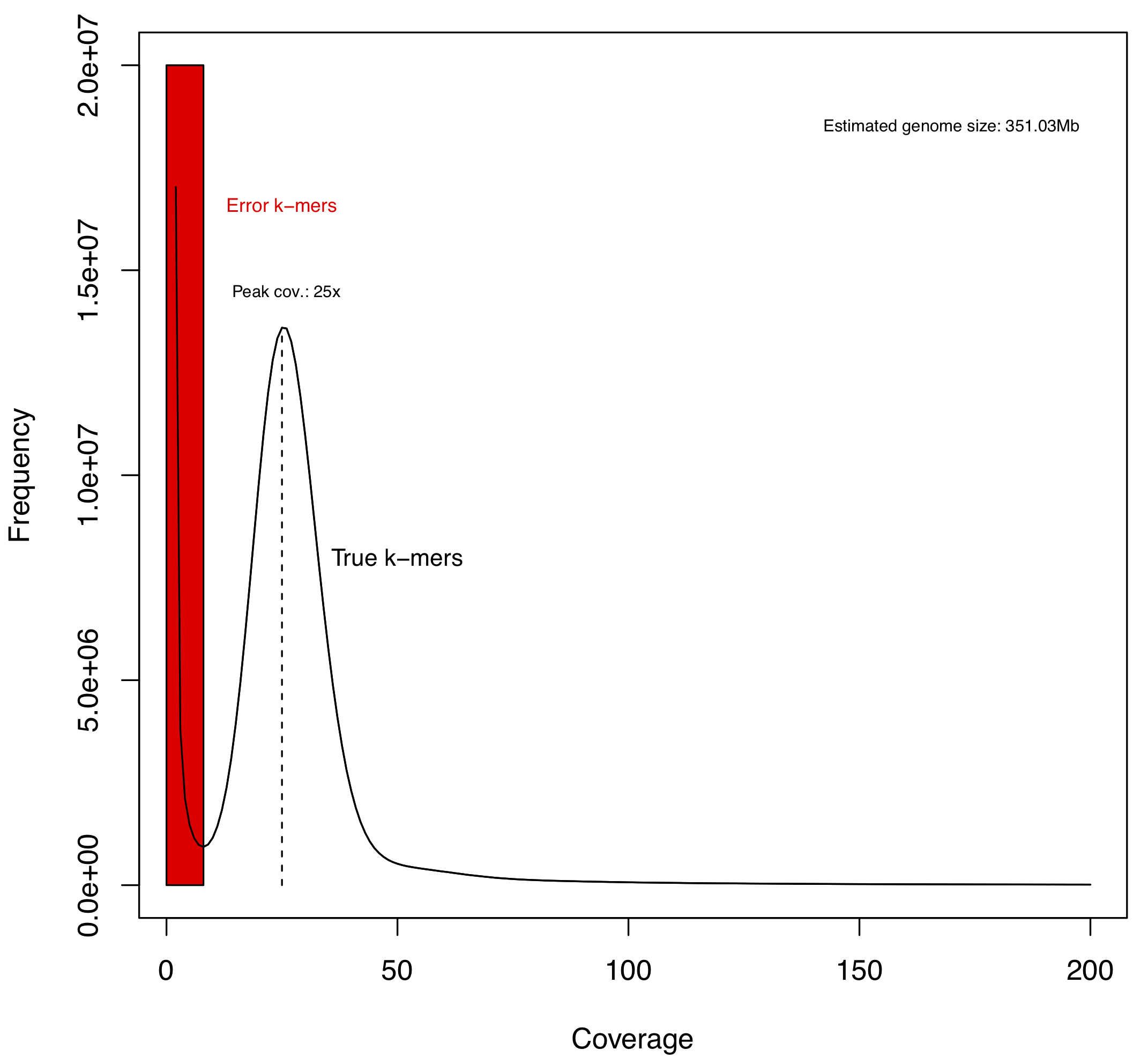
Figure 6.5: Distribution of 21-mer frequencies based on the trimmed library with insert fragment size of 180 bp. Given only one peak in the k-mer distribution, we predict that the Apostasia shenzhenica genome has limited heterozygosity or in other words, that this genome is inbred.
6.8.7.2.2 K-mer graph and PCR effect
The peak around 25 in Figure 6.5 is the coverage with the highest number of different 21-mers. This means that there are \(1.4e^7\) unique 21-mers (frequency) that have been observed 25 times (coverage). The normal-like distribution is due to the fact that the sequencing did not provide a perfect coverage of the whole genome. Some regions have less coverage, whereas others have a little more coverage, but the average coverage depth is around 25.
The large number of unique k-mers (\(1.7e^7\)) that have a frequency of 1 (right left side of the graph; Figure 6.5) is most likely due to PCR errors. Please find below an example explaining how PCR errors impact on the k-mer procedure.
All 3-mers of the sequence “AATTGGCCG” are:
- AAT, ATT, TTG, TGG, GGC, GCC, CCG
Now, let’s consider that the 4th letter (T) in the sequence above is replaced with a C to simulate a PCR error. In this context, all 3-mers of this sequence “AATCGGCCG” are:
- AAT, ATC, TCG, CGG, GGC, GCC, CCG.
The k-mers in bold are the incorrect 3-mers that are now unique and end up at the beginning of the graph in Figure 6.5.
Overall, the general rule is that for a given sequence, a single PCR error will result in \(k\) unique and incorrect k-mers.
6.8.7.3 Bioinformatics
Please follow the approach below to:
- Trim reads based on Phred quality scores
- Normalize high coverage reads, remove PCR errors and low quality reads
- Remove intermediate files
- Prepare data for de novo genome assembly
- Reads QCs on cleaned reads
Note: Perform the analyses in your tmux session entitled Part1.
6.8.7.3.1 Trim reads based on Phred quality scores
Let’s start the cleaning of our interleaved PE reads by trimming reads using Phred scores (33) as implemented in seqtk.
Before executing the commands below do the following:
- Attach to your Part1
tmuxsession - Navigate to
~/Documents/02_Kmers_analyses/khmerusingcd - Type to following command:
- Input:
SRR5759389_pe12.fastq - Output:
SRR5759389_pe12.trimmed.fastq
#Trim reads based on Phred scores (default of 33)
# --> This code uses the raw Illumina data deposited on our shared folder
seqtk trimfq /home/Genomics_shared/Chapter_04/01_SRA/SRR5759389_pe12.fastq > SRR5759389_pe12.trimmed.fastq
Using Phred scores to clean our data is not going to deal with PCR errors and potential effects of high repeated DNA sequences on the de novo assembly. Below, we will use information on k-mer distributions to address these issues and clean our dataset accordingly.
6.8.7.3.2 Normalize high coverage reads and filter low abundance reads based on k-mer frequencies
In the next commands, khmer (Crusoe et al., 2015) will be used to:
- Normalize high coverage reads (>100x) based on median coverage (to optimize RAM requirements for de novo genome assembly).
- Filter low abundance reads (most likely PCR errors).
- Final clean-up of reads to remove low quality bases, short sequences, and non-paired reads
To conduct these analyses, run the following commands in your Part1 tmux session (you should be in ~/Documents/02_Kmers_analyses/khmer):
- Normalize high coverage reads (>100x) based on median reads coverage using k-mer frequencies
- Input:
SRR5759389_pe12.trimmed.fastq - Output:
SRR5759389_pe12.max100.trimmed.fastq
# Normalize high coverage reads (>100x)
khmer normalize-by-median.py -p --ksize 21 -C 100 -M 1e9 -s kmer.counts -o SRR5759389_pe12.max100.trimmed.fastq SRR5759389_pe12.trimmed.fastq- Filter low abundance reads based on k-mer frequencies to minimize PCR errors
- Input:
SRR5759389_pe12.max100.trimmed.fastq - Output:
SRR5759389_pe12.max100.trimmed.norare.fastq
# Filter low abundance reads based on k-mer frequencies to minimize PCR errors
khmer filter-abund.py -V kmer.counts -o SRR5759389_pe12.max100.trimmed.norare.fastq SRR5759389_pe12.max100.trimmed.fastq
6.8.7.3.3 Final clean-up of reads
Final clean-up of reads to remove low quality bases, short sequences, and non-paired reads
- Input:
SRR5759389_pe12.max100.trimmed.norare.fastq - Output:
SRR5759389_pe12.max100.trimmed.norare.noshort.fastq
# Final clean-up of reads (remove low quality bases, short sequences, and non-paired reads)
seqtk seq -q 10 -N -L 80 SRR5759389_pe12.max100.trimmed.norare.fastq | seqtk dropse > SRR5759389_pe12.max100.trimmed.norare.noshort.fastq
6.8.7.3.4 Remove intermediate files
To save disk space and avoid cluttering the computer (with redundant information), please remove the following intermediate files as follows uisng the rm command:
#Removing intermediate, temporary files to save disk space
rm SRR5759389_pe12.max100.trimmed.fastq
rm SRR5759389_pe12.max100.trimmed.norare.fastq
–> Each of the file that you discarded is >30G of data!
6.8.7.3.5 Prepare data for de novo genome assembly
In this last section, our cleaned reads are prepared for the de novo genome assembly analysis conducted in SOAPdenovo2 (Luo et al., 2012) (done in PART 2). This is achieved by using khmer to de-interleave reads and rename files using mv as follows:
- De-interleave filtered reads (to be ready for de novo assembly in SOAPdenovo2)
- Input:
SRR5759389_pe12.max100.trimmed.norare.noshort.fastq - Output:
- R1:
SRR5759389_pe12.max100.trimmed.norare.noshort.fastq.1 - R2:
SRR5759389_pe12.max100.trimmed.norare.noshort.fastq.2
- R1:
# De-interleave filtered reads
khmer split-paired-reads.py SRR5759389_pe12.max100.trimmed.norare.noshort.fastq- Rename output reads to something more human-friendly
- Input:
- R1:
SRR5759389_pe12.max100.trimmed.norare.noshort.fastq.1 - R2:
SRR5759389_pe12.max100.trimmed.norare.noshort.fastq.2
- R1:
- Output:
- R1:
SRR5759389.pe1.clean.fastq - R2:
SRR5759389.pe2.clean.fastq
- R1:
#Rename output reads
mv SRR5759389_pe12.max100.trimmed.norare.noshort.fastq.1 SRR5759389.pe1.clean.fastq
mv SRR5759389_pe12.max100.trimmed.norare.noshort.fastq.2 SRR5759389.pe2.clean.fastq
–> These final files are the input files for the de novo analysis.
6.8.7.3.6 Reads QCs on cleaned reads
Use FastQC to validate the reads cleaning conducted above. Please see Step 2 for more details on the methodology.
6.8.8 Step 4: What’s “in” the reads?
After inspecting the output of the reads QC analyses, we discovered that our Illumina library contained two distinct sequence content patterns. This evidence together with the nature of the organism that we are studying allowed us to hypothesize that our data were enriched in plastid (or chloroplast) DNA over nuclear DNA. In this context, we predict that the 32x sequencing nuclear genome coverage inferred based on the raw data could be significantly lower. To test our hypothesis and determine the actual sequencing coverage of the nuclear genome, it is paramount to:
- Determine whether the data are contaminated
- Provide an estimate of the proportions of reads belonging to either nuclear or chloroplast genomes.
6.8.8.1 Analytical workflow
To investigate these topics, the instructor proposes that we conduct the following analyses:
6.8.8.2 Input data
All the analyses from this step rely on SRR5759389_pe12.max100.trimmed.norare.noshort.fastq. If you have not been able to generate the latter file, please copy it from our shared hard drive space into your khmer/ folder. The path is as follows:
## SRR5759389_pe12.max100.trimmed.norare.noshort.fastq
# can be found at this path
/home/Genomics_shared/Chapter_04/02_Kmers_analyses/khmer/instructor_files
6.8.8.3 Group work
Students are divided into 3-4 small groups. Each group work as a team to conduct the analyses and answer questions. Prior to assigning tasks, the group has to work on a workflow describing the analyses (input/output), used software (and arguments) and carefully reading the material prior to running jobs in secured tmux sessions.
6.8.8.4 Reads GC contents
The GC content of a sequence library can provide evidence of contamination or the presence of sequence from multiple organisms (since most organisms have specific GC profiles). A GC plot inferred from a non-contaminated library would display a smooth, uni-modal distribution. The existence of shoulders, or in more extreme cases a bi-modal distribution, could be indicative of the presence of sequence reads from an organism with a different GC content, which is most likely a contaminant (see Figure 6.3).
6.8.8.4.1 Bioinformatics
Here we infer GC contents for all clean reads using the perl script GC_content.pl. This script requires reads to be in fasta format. We will then start by converting our fastq file into fasta by using seqtk. Data are available in the ~/Documents/02_Kmers_analyses/GC_content/ folder. Please see below for the commands to be executed:
- Convert clean reads from
fastqtofasta
- Input:
SRR5759389_pe12.max100.trimmed.norare.noshort.fastq - Output:
SRR5759389_pe12.max100.trimmed.norare.noshort.fasta
#Convert fastq to fasta
seqtk seq -a ~/Documents/02_Kmers_analyses/khmer/SRR5759389_pe12.max100.trimmed.norare.noshort.fastq > SRR5759389_pe12.max100.trimmed.norare.noshort.fasta- Infer GC content of all cleaned reads in
fastaformat
- Input:
SRR5759389_pe12.max100.trimmed.norare.noshort.fasta - Output:
gc_out.txt–> Don’t execute command and just use this file for next analyses
PLEASE DON’T EXECUTE THE COMMAND BELOW! It takes few hours to calculate reads GC contents. Use the output of this command gc_out.txt (weighing ca. 5GB), which is available in the GC_content/ folder to carry on our analyses.
#Infer GC content using fasta file as input (this can take a long time)
./GC_content.pl SRR5759389_pe12.max100.trimmed.norare.noshort.fasta > gc_out.txt- Mine reads GC content in large file
- Input:
gc_out.txt - Output:
gc_simple.txt
The next command extracts the column containing the GC content per read from gc_out.txt (located in GC_content/). Since the file is very big, we use the BASH command awk to extract this information instead of R.
#Extract reads GC contents (the file is big and can't be processed easily)
awk '{print$2}' gc_out.txt > gc_simple.txt- Infer histogram of GC contents in cleaned library
- Input:
gc_simple.txt - Output:
GC_content_hist.pdf
The last part of the analysis will be executed in R where we will load the data and create a histogram to look at the distribution of reads GC contents.
### ~~~ Infer GC content per reads ~~~ Load the data in R
gc_frac <- read.table("gc_simple.txt", header = T)
# Create pdf to save output of hist
pdf("GC_content_hist.pdf")
# Do the histogram of GC content
hist(as.numeric(gc_frac[, 1]), main = "Histogram of GC content per reads",
    xlab = "GC fraction")
# Close pdf file
dev.off()
The histogram displaying the distribution of GC values based on cleaned reads is provided in Figure 6.6.
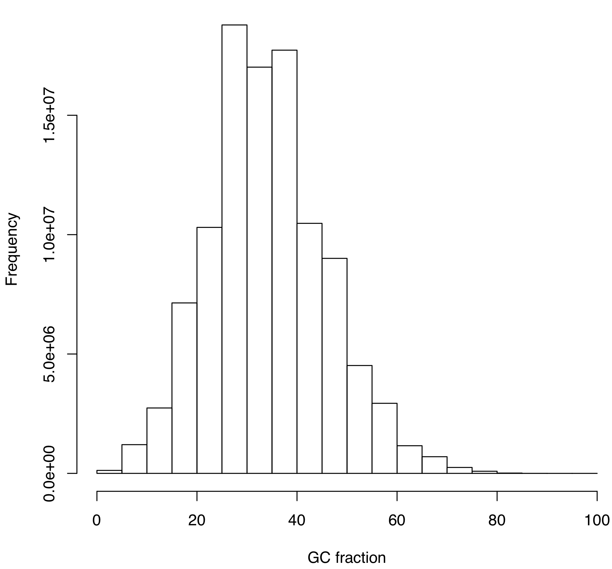
Figure 6.6: Histogram of GC values inferred from the cleaned library of reads (SRR5759389). See text for more details.
6.8.8.4.2 Question
To your knowledge, based on data presented in Figure 6.6, is the SRR5759389 library contaminated with alien DNA?
6.8.8.5 Mapping reads against reference genomes
Here we aim at assessing the proportions of reads in the clean library belonging to either nuclear or chloroplast genomes by mapping our clean reads against two reference genomes using bwa (Li and Durbin, 2009) and samtools (Li, Handsaker, et al., 2009). Data are available in Map_reads/.
6.8.8.5.1 Mapping reads against the nuclear genome
The nuclear genome of Apostasia shenzhenica published by Zhang et al. (2017) is not listed in the NCBI database as “Genome”, but rather as “Assembly” (see BioProject PRJNA310678). Please see Figure 6.7 for more details on the genome. This file (a compressed FASTA) is already available in your folder, but you could download it as follows:
#Get Fasta files for genomes of reference
#PEFY01 nuclear genome of Apostasia
wget ftp://ftp.ncbi.nlm.nih.gov/sra/wgs_aux/PE/FY/PEFY01/PEFY01.1.fsa_nt.gz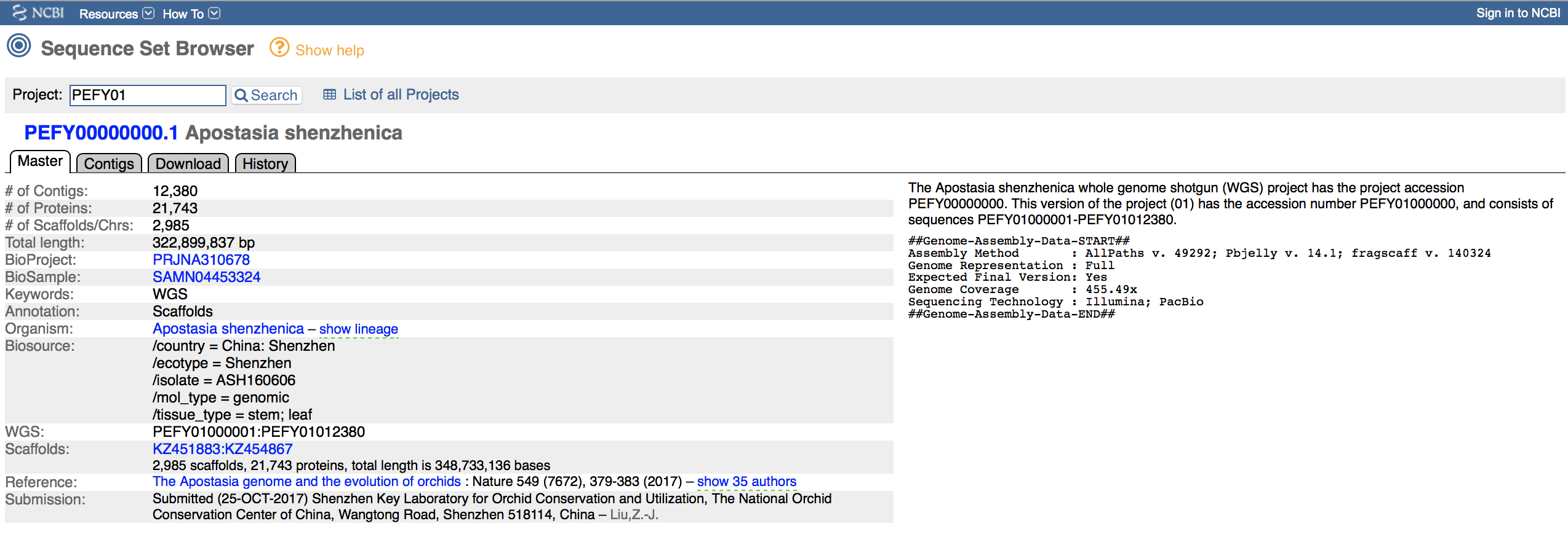
Figure 6.7: Screen shot of the NCBI website showing details about the accession containing the nuclear genome assembly of Apostasia shenzhenica under the accession PEFY01.
6.8.8.5.2 Bioinformatics
Please go through the commands below to map your clean reads against the reference nuclear genome assembly:
- Map
fastqcleaned reads to nuclear reference genome assembly (infasta) usingbowtie
- Input:
SRR5759389_pe12.max100.trimmed.norare.noshort.fastqandPEFY01.1.fsa_nt.gz - Output:
PEFY01_map_pe.sorted.bam- This file will be used as input for counting reads
#Mapping clean reads against reference genome using bwa and converting into human readable format using samtools

#Before starting, you have to create an index for your reference genome to allow efficient mapping
bwa index -a bwtsw PEFY01.1.fsa_nt.gz
bwa mem -t 20 PEFY01.1.fsa_nt.gz ~/Documents/02_Kmers_analyses/khmer/SRR5759389_pe12.max100.trimmed.norare.noshort.fastq | samtools view -buS - | samtools sort - -o PEFY01_map_pe.sorted.bam
samtools index PEFY01_map_pe.sorted.bam
We will be devoting time to decipher these commands during our Lab sessions. For now, here is a short description of bwa from the manual:
BWA is a software package for mapping low-divergent sequences against a large reference genome, such as the human genome. It consists of three algorithms: BWA-backtrack, BWA-SW and BWA-MEM. The first algorithm is designed for Illumina sequence reads up to 100bp, while the rest two for longer sequences ranged from 70bp to 1Mbp. BWA-MEM and BWA-SW share similar features such as long-read support and split alignment, but BWA-MEM, which is the latest, is generally recommended for high-quality queries as it is faster and more accurate. BWA-MEM also has better performance than BWA-backtrack for 70-100bp Illumina reads.
6.8.8.5.3 Mapping reads against the chloroplast genome
The chloroplast genome of Apostasia shenzhenica was not published. To assess the proportion of chloroplastic reads in our Illumina cleaned reads, we will use the chloroplast genome of a sister species, A. wallichii (Niu et al., 2017), which is available on the NCBI website under the accession number LC199394. This file (in FASTA) is already available in your folder and you do not have to download it.
6.8.8.5.4 Bioinformatics
Please execute the commands below to map the clean reads against the reference chloroplast genome of the sister species:
- Map
fastqcleaned reads to chloroplast genome assembly (infasta) usingbowtie
- Input:
SRR5759389_pe12.max100.trimmed.norare.noshort.fastqandLC199394.fasta - Output:
LC199394_map_pe.sorted.bam- This file will be used as input for counting reads
#Mapping reads against the chloropolast genome of a sister species
# following the same approach as with the nuclear genome
bwa index -a bwtsw LC199394.fasta
bwa mem -t 20 LC199394.fasta ~/Documents/02_Kmers_analyses/khmer/SRR5759389_pe12.max100.trimmed.norare.noshort.fastq | samtools view -buS - | samtools sort - -o LC199394_map_pe.sorted.bam
samtools index LC199394_map_pe.sorted.bam
6.8.8.5.5 Counting reads belonging to nuclear and chloroplast genomes
We have now all the information at hand to count how many reads are matching with either nuclear or chloroplast genomes (and infer proportions). Remember that it is just a very preliminary assessment, which aims at assessing the quality of the library and its suitability for de novo genome assembly.
6.8.8.5.6 Bioinformatics
- Count the total number of cleaned reads using
count_fastq.sh
- Input:
SRR5759389_pe12.max100.trimmed.norare.noshort.fastq - Output: A number echoed on the screen.
#Count the total number of clean reads
./count_fastq.sh ~/Documents/02_Kmers_analyses/khmer/SRR5759389_pe12.max100.trimmed.norare.noshort.fastq- Count the number of cleaned reads mapping to each genome
- Input:
PEFY01_map_pe.sorted.bamandLC199394_map_pe.sorted.bam - Output: Two numbers (one per command) echoed on the screen.
Now, we will use samtools to count how many unique reads mapped the reference genomes:
#How many unique reads mapped the nuclear genome
samtools view -F 0x904 -c PEFY01_map_pe.sorted.bam

#How many unique reads mapped the chloroplast genome
samtools view -F 0x904 -c LC199394_map_pe.sorted.bam- Infer the proportion of cleaned reads belonging to each genome
The instructor let you work on code to determine these values.
6.8.8.5.7 Questions
What are the proportions of nuclear and chloroplast reads in your library as well as potential contaminants?
Based on your previous answer, is this library suitable to assemble the nuclear genome of Apostasia shenzhenica?
6.8.9 Step 5: Estimate genome size and other genomic features
6.8.9.1 Aim
In this section, we aim at utilizing data on k-mer frequencies to estimate the nuclear genome size and tease apart the proportion of the genome associated with low copy genes (also referred to as unique sequences) and repetitive DNA.
6.8.9.2 Methodology
The JELLYFISH (Marçais and Kingsford, 2011) program is a tool for fast, memory-efficient counting of k-mers in DNA sequences. JELLYFISH is a command-line program that reads FASTA and multi-FASTA files containing DNA sequences and it outputs k-mer counts in an binary format (which can easily be translated into a human-readable text). Finally, the output of JELLYFISH will be used to estimate the genome size and complexity of the Apostasia shenzhenica nuclear genome by using R and GenomeScope (Vurture et al., 2017).
6.8.9.3 Group work
In this section, the JELLYFISH analysis has to be done in groups, but the rest of the analyses (in R and with GenomeScope) can be done individually.
6.8.9.4 Generate countings of k-mers
Here, we are using JELLYFISH to generate countings of 21-mers based on the cleaned Illumina reads (SRR5759389_pe12.max100.trimmed.norare.noshort.fastq). We will subsequently input the output of this program into R to estimate the genome size based on k-mer frequencies.
The data are available in Jellyfish/ and all analyses must be done in your tmux Part1 session.
- Input:
SRR5759389_pe12.max100.trimmed.norare.noshort.fastq - Output:
Orchid_21mer_SRR5759389_pe12_max100.trimmed.norare.histo
Note: This job uses 30 CPUs (or Central Processing Units) to infer k-mers and it would be best to work in groups to execute these tasks.
# 1. Navigate to the right folder (Jellyfish/) using cd

# 2. Run jellyfish to obtain k-mer counts and frequencies (based on trimmed, normalized and filtered reads)
jellyfish count -t 30 -C -m 21 -s 5G -o Orchid_21mer_SRR5759389_pe12_max100.trimmed.norare ~/Documents/02_Kmers_analyses/khmer/SRR5759389_pe12.max100.trimmed.norare.noshort.fastq

jellyfish histo -o Orchid_21mer_SRR5759389_pe12_max100.trimmed.norare.histo Orchid_21mer_SRR5759389_pe12_max100.trimmed.norare
Note: To ensure that everybody can run the rest of the analyses on their own, copy Orchid_21mer_SRR5759389_pe12_max100.trimmed.norare.histo into the shared folder at this path:
/home/Genomics_shared/Chapter_04/02_Kmers_analyses/
Each member of the group will then copy this file over to their account (at the right path) to pursue the analyses.
6.8.9.5 Infer genome size with R
Once the JELLYFISH analysis is completed, please open an R session and execute the following command to estimate the haploid (1x) genome size. Here, genome size is estimate as follows:
#Genome size (N) is equal to:
N = Total numbers of k-mers / Peak of coverage (here ca. 22x)
N = Area under the curve / Peak of coverage
The R script to infer the genome size of Apostasia shenzhenica based on the data generated by JELLYFISH is presented below:
# 1. Load the output of Jellyfish in R
Clean <- read.table("Orchid_21mer_SRR5759389_pe12_max100.trimmed.norare.histo")
# 2. Execute this user defined function to infer genome
# size and plot k-mer distribution A function to infer
# genome size (1C or haploid) on jellyfish output input -
# hist = table containing output of Jellyfish (hist file) -
# plotKmers if 'TRUE' outputs a graph
GenomeSize <- function(hist, plotKmers) {
    # Infer Genome size
    x <- grep(min(hist[1:20, 2]), hist[, 2])
    tmp <- hist[x:1000, 1] * hist[x:1000, 2]
    # Infer the total number of kmers in the distribution
    Totkmers <- sum(as.numeric(as.vector(tmp)))
    # Infer Peak of coverage (when enough data is equal to
    # mean) of the genome (13x)
    PeakCov <- grep(max(hist[x:1000, 2]), hist[, 2])
    # Genome size (1C or haploid) is the area under the
    # curve, which is the Total numner of K-mers/Mean
    # coverage
    GenomeSizeOut <- Totkmers/PeakCov
    GenomeSizeOut <- round(GenomeSizeOut/1e+06, 2)
    print(GenomeSizeOut)
    if (plotKmers == "TRUE") {
        # Plot
        plot(hist[2:200, ], type = "n", ylim = c(0, 2e+07), xlab = "Coverage",
            ylab = "Frequency", main = "K-mer (k=21) distribution")
        # Plot trimmed data
        lines(hist[2:200, ])
        # These are low coverage K-mers (K=1:8), which have
        # very high frequencies
        rect(xleft = 0, ybottom = 0, xright = x, ytop = 2e+07,
            col = "red")
        text(x = 25, y = hist[PeakCov, 2] + 3e+06, paste("Error k-mers",
            sep = "\n"), cex = 0.7, col = "red")
        # Add the distribution line
        lines(hist[2:200, ], type = "l")
        # Add a line showing the peak of coverage (here at
        # 26x)
        segments(x0 = PeakCov, y0 = 0, x1 = PeakCov, y1 = hist[PeakCov,
            2], lty = 2)
        text(x = 26, y = hist[PeakCov, 2] + 9e+05, paste("Peak cov.: ",
            PeakCov, "x", sep = ""), cex = 0.6)
        text(x = 50, y = 8e+06, paste("True k-mers", sep = "\n"),
            cex = 0.8)
        text(x = 170, y = 18500000, paste("Estimated genome size: ",
            GenomeSizeOut, "Mb", sep = ""), cex = 0.6)
    }
}
# 3. Estimate genome size on cleaned reads using the
# function GenomeSize
pdf("GenomeSize.pdf")
GenomeSize(Clean, plotKmers = "TRUE")
dev.off()
6.8.9.6 Transfer files onto your personnal computer
Please use FileZilla or the sftp protocol (if you have a UNIX-based OS) to transfer GenomeSize.pdf and Orchid_21mer_SRR5759389_pe12_max100.trimmed.norare.histo onto your personal computer. The latter file will be required to conduct the GenomeScope analysis (see below).
6.8.9.7 Questions
What is the haploid genome size of Apostasia shenzhenica?
How does this genome size estimation compare with the one conducted based on reads that were only trimmed provided in Figure 6.5?
Finally, are the latter two estimations close to the 349 Mb provided in Zhang et al. (2017)?
6.8.9.8 Use GenomeScope to estimate heterozygosity, unique genes, repetitive DNA and PCR errors
6.8.9.8.1 Aim
Finally, the last step of our preliminary analyses prior to de novo genome assembly aims at estimating heterozygosity, unique genes, repetitive DNA and PCR errors. These analyses are conducted by using the approach implemented in the online tool GenomeScope (Vurture et al., 2017). The authors of this program developed an equation to model the shape and size of the k-mer graph by using four negative binomial peaks which shape and size are determined by % heterozygosity, % PCR duplication, and % PCR Error.
6.8.9.8.2 Bioinformatics
Open a web browser and navigate to the GenomeScope website (http://qb.cshl.edu/genomescope/). Once on the website, upload Orchid_21mer_SRR5759389_pe12_max100.trimmed.norare.histo by dragging your file onto the small window and set the analysis as provided in Figure 6.8.
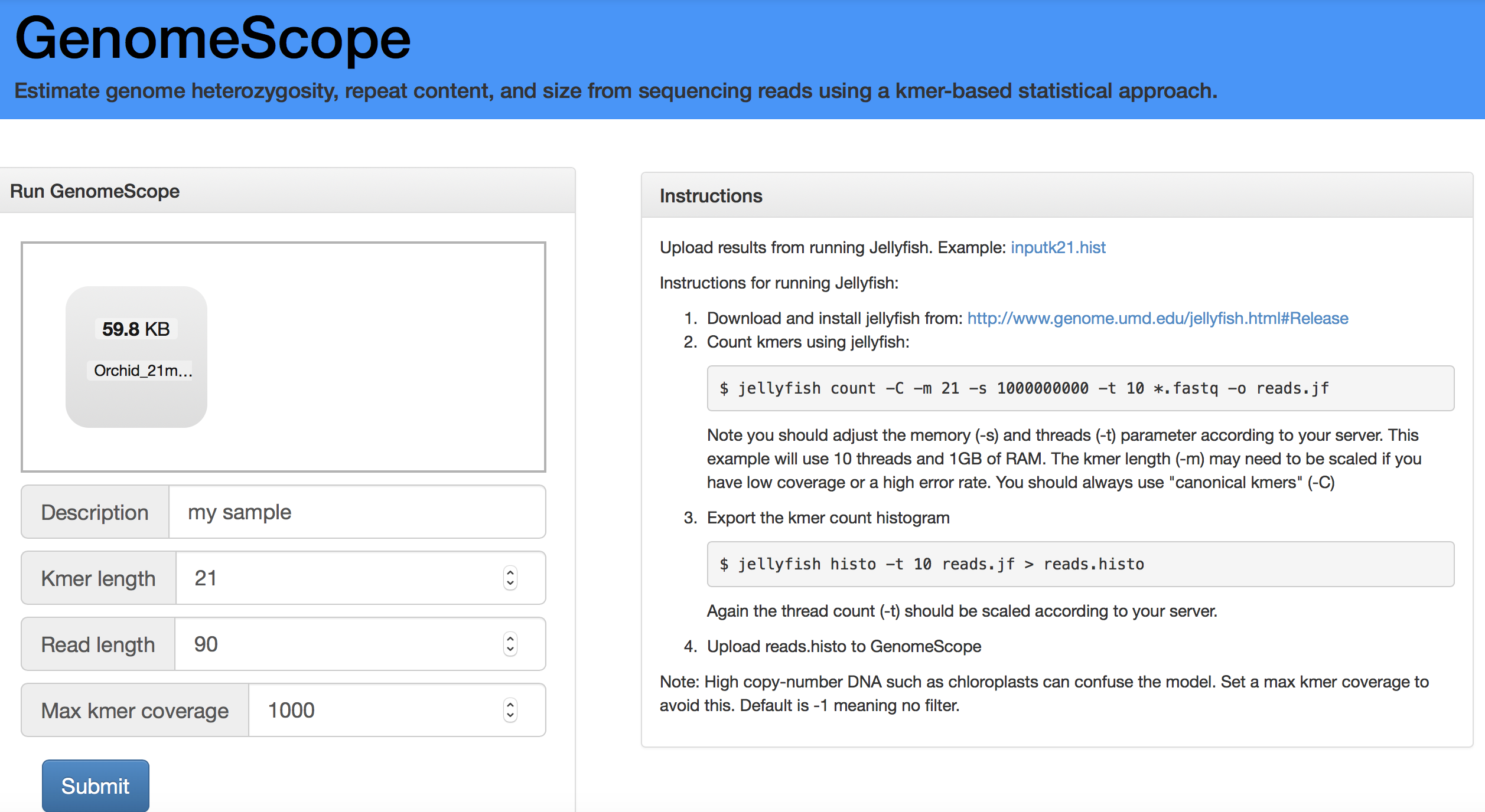
Figure 6.8: Screen shot of the GenomeScope portal to help you setting your analysis.
6.8.9.8.3 Interpreting results of GenomeScope
The output of GenomeScope is displayed in Figure 6.9. The program outputs two plots and the only difference between those is that the the second plot is using a log transformation for the axes. This transformation allows better teasing apart the different elements studied here. The big peak at 25 in the graph above is in fact the diploid homozygous (i.e., AA) portions of the genome that account for the identical 21-mers from both strands of the DNA (haploid genome mostly composed of single-copy genes). The dotted line corresponds to the predicted center of that peak. The absence of a shoulder to the left of the peak suggests that this genome has a very low level of heterozygosity (i.e., AB). The red line on the left corresponds to PCR errors. Finally, the proportion of unique sequences, which would correspond to low-copy genes is depicted by the yellow line and the amount of repetitive DNA is estimated by comparing the “space” between the black and yellow lines (on the right side of the graph).
Please see this tutorial for more information on the model implemented in GenomeScope and interpretation of the results.
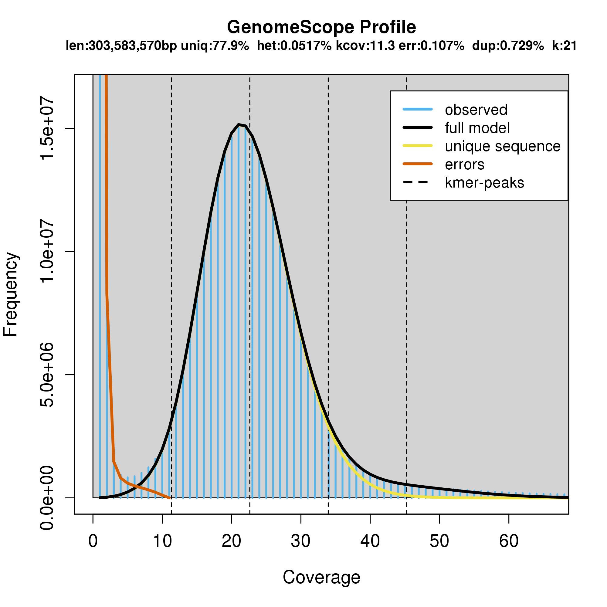
Figure 6.9: Output of the GenomeScope analysis.
6.8.9.9 Questions
How do estimations of genome size differ between R and GenomeScope?
What is the level of genomic heterozygosity of Apostasia shenzhenica?
Is the genome of Apostasia shenzhenica enriched in repeats?
6.9 PART 2: De novo genome assembly
6.9.1 Objective
The overarching objective of PART 2 is to gain theoretical and bioinformatics knowledge on the steps required to perform a de novo genome assembly based on cleaned Illumina reads. The procedure applied to assess and validate the quality of the genome assembly will also be covered in PART 3.
6.9.2 Presenting the data and their location
PART 2 will be using the output files of the PART 1 reads cleaning step, which are deposited in ~/Documents/02_Kmers_analyses/khmer/ and named as follows:
SRR5759389.pe1.clean.fastqSRR5759389.pe2.clean.fastq
WARNING: You have to complete section 6.8.7.3.5 before starting this section.
6.9.3 Analytical workflow
To achieve our overarching objective, our next classes will be divided into two steps:
- Step 1: Set-up and perform a de novo genome assembly based on cleaned paired-end (PE) Illumina reads using
SOAPdenovo2(Luo et al., 2012). - Step 2: Provide theoretical knowledge on de novo genome assembly methods by focusing on de Bruijn graphs.
6.9.4 Step 1: Perform de novo genome assembly analysis
6.9.4.1 Specific objective
Here, students will be learning the procedure to set-up and perform a de novo genome assembly using cleaned PE Illumina reads as implemented in SOAPdenovo2 (Luo et al., 2012). The analysis will be conducted on the output files obtained after cleaning reads based on Phred scores and k-mer distributions (see section 6.9.2 for more details on the input files).
SOAPdenovo2 is the updated version of the program that was used by Li, Fan, et al. (2009) to assemble the nuclear genome of the giant panda. The draft nuclear genome of Apostasia shenzhenica was not inferred with this latter program, but with ALLPATHS-LG (Gnerre et al., 2011). The draft assembly was obtained based on multiple Illumina short-reads libraries exhibiting different insert-sizes (see Zhang et al., 2017). The authors have conducted a final round of gap closures to polish their assembly based on PacBio long-reads. It will therefore be interesting to compare our assembly based on one Illumina library with the one obtained by Zhang et al. (2017) inferred uisng a combination of short and long read data. Further information justifying using SOAPdenovo2 instead of ALLPATHS-LG are provided below.
6.9.4.2 Background on SOAPdenovo2
SOAPdenovo2 (Luo et al., 2012) is a short-read genome assembler, which was especially developed to handle Illumina reads and to build de novo draft assemblies for human-sized genomes. This program creates new opportunities for building reference sequences and carrying out accurate analyses of unexplored genomes in a cost effective way. As stated above, SOAPdenovo2 aims for large eukaryote genomes, but it also works well on bacteria and fungi genomes. It runs on 64-bit Linux system with a minimum of 5GB of physical memory. For big genomes like human (3.2Gbp), about 150GB of memory are required.
In our case, we have estimated the haploid genome size of Apostasia shenzhenica to be around 340Mbp in our previous tutorial. This latter evidence therefore suggests that is adapted to assemble a draft genome for this species of orchid.
6.9.4.3 Structure of SOAPdenovo2
This program is made up of six modules handling:
- Read error correction.
- de Bruijn graph construction.
- Contig assembly.
- Paired-end reads mapping.
- Scaffold construction.
- Gap closure.
Please read Luo et al. (2012) for more details on the approach implemented in SOAPdenovo2.
6.9.4.4 Why are we using SOAPdenovo2 to assemble this genome?
Once reads are fully cleaned and ready for de novo assembly, one of the main questions that you will ask yourself is: What de novo program should I use to assemble my genome? Or in other words, which program best fit my data?
Most researchers working on Illumina short-reads are using either SOAPdenovo2 or ALLPATHS-LG to assemble nuclear genomes of eukaryote species. Please find below a short comparison of both programs:
- Unlike
SOAPdenovo2,ALLPATHS‐-LGrequires high sequence coverage of the genome in order to compensate for the shortness of the Illumina reads. The precise coverage required depends on the length and quality of the paired reads, but typically is of the order 100x or above. This is raw read coverage, before any error correction or filtering. - Unlike
SOAPdenovo2,ALLPATHS‐-LGrequires a minimum of 2 paired-end libraries – one short and one long. The short library average separation size must be slightly less than twice the read size, such that the reads from a pair will likely overlap – for example, for 100 base reads the insert size should be 180 bases. The distribution of sizes should be as small as possible, with a standard deviation of less than 20%. The long library insert size should be approximately 3000 bases long and can have a larger size distribution. Additional optional longer insert libraries can be used to help disambiguate larger repeat structures and may be generated at lower coverage.
Overall, because we estimated in the previous tutorial that this library provided a coverage depth of ca. 25x for the haploid genome and that we only have one paired-end library, SOAPdenovo2 therefore best fits our data.
6.9.4.5 Running SOAPdenovo2 analysis
Running a SOAPdenovo2 analysis is a three steps process:
- Step 1: Create a folder and move the de-interleaved cleaned paired-end ‘fastq’ files.
- Step 2: Create a
SOAPdenovo2configuration file providing settings for the analysis. - Step 3: Run the de novo genome assembly analysis.
Run the code in a tmux session!
6.9.4.5.1 Step 1
Use the mkdir command to create a new folder entitled SOAPdenovo/ in ~/Documents/02_Kmers_analyses/ as follows:
mkdir SOAPdenovo2Move the paired-end cleaned reads files (i.e. input files for the de novo analysis) in SOAPdenovo2/ using the mv command as follows:
#Move the split pe files in SOAPdenovo2
# WARNING: You have to be in the SOAPdenovo2 folder
mv ../khmer/SRR5759389.pe* .
6.9.4.5.2 Step 2
SOAPdenovo2 requires a configuration file to run the analysis.
Please create a file entitled soap_config.txt deposited in SOAPdenovo2/ using vim.
- Type the following command in the terminal, which will create the new file and open a
vimsession:
vim soap_config.txtType
ShiftandIon your keyboard to enter intoINSERTmode.Copy and paste the text below in the
vimsession:
max_rd_len=90          # maximal read length
[LIB]            # One [LIB] section per library
avg_ins=180             # average insert size
reverse_seq=0           # if sequence needs to be reversed
asm_flags=3             # use for contig building and subsequent scaffolding
rank=1                  # in which order the reads are used while scaffolding
q1=SRR5759389.pe1.clean.fastq
q2=SRR5759389.pe2.clean.fastq
To better understand the settings contained in this file, comments have been provided to explain each parameter. The last 2 lines contain the names of the input files. This is a very simple analysis based only on one paired-end Illumina library ([LIB]).
- Hit
Escon your keyboard to quit theINSERTmode and type:wq!to save the document and exit fromvim.
6.9.4.5.3 Step 3
Once the input and configuration files are sorted, just type the following command in your terminal to start the analysis:
#Run the de novo analysis
soapdenovo2-63mer all -s soap_config.txt -K 63 -R -p 5 -o SRR5759389_assembly
Here, SOAPdenovo2 works with a k-mer size of 63 (-K). The analysis will be performed on 5 threads (or CPUs) (-p) and the program will save the output files under SRR5759239_assembly as shown by the -o argument.
The analysis will run for SEVERAL HOURS. Please log out from your sessions, but DON’T SWITCH OFF COMPUTERS.
The output file of the SOAPdenovo2 analysis are presented in section 6.10.2.
6.10 PART 3: Validation of the draft genome
6.10.1 Objective
In this part, students are learning how to use QUAST to assess the quality of the de novo genome assembly inferred in PART 2 using SOAPdenovo2.
QUAST is used to validate the assembly (based on one PE Illumina library; SRR5759389) by comparing it with the assembly published by Zhang et al. (2017) (available under the GenBank accession number: PEFY01). Such approach is especially useful to assess the level of misassembly (see Figure 6.10). Please keep in mind that this assembly has only been inferred from one PE Illumina library.
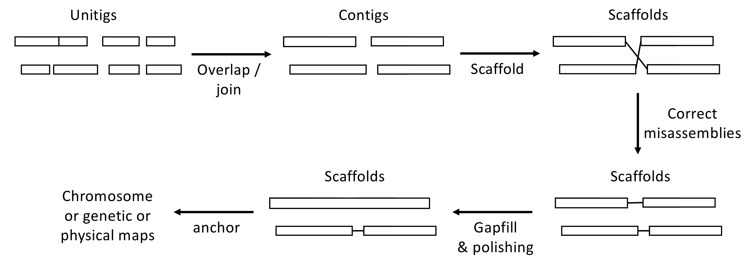
Figure 6.10: Overview of the assembly workflow. Here are few key definitions: Contig: A contiguous sequence of bases. Unitig: A type of contig for which there are no competing choices in terms of internal overlaps (they usually stop before a repeat sequence). Scaffold: A sequence of contigs separated by gaps (Ns). See PART 2 for more details.
6.10.2 SOAPdenovo2 assembly files
The input of the QUAST analysis is the fasta assembly file produced by SOAPdenovo2 containing scaffolds (see Figure 6.10). This file is entitled SRR5759389_assembly.scafSeq and it is located in the SOAPdenovo2/ folder (see PART 2 for more details).
6.10.2.1 Inspecting assembly files
Navigate to the file location and inspect SRR5759389_assembly.scafSeq by using the head command. It should be similar to the example provided below:
>scaffold2  6.9
TATATATATTAGCATTAAATTAACTTTATTTTCATTCTTTCACAAAGCTCGAAACAAAGAT
ATCACCAAACAACTATGGCTTAGCAAACACATCATTTATACGAGAAATATTAACGATTTG
AGTGGTGTATGTAGGTTTATGTTCTGAAGTTAACTCGCCCTTTTTTTTTTTTTTCTTAAGT
ACTGATTNNNNNNNNNNNNNNNNNNNNNNNNNNNNNNNNNNNNNNNNTTCTTCTTCT
TCTAATCATAATATATGTGGTGCTTGCATTTGTGTGCCATGGTGTCACCCTCCCTTCTTG
CATTGGCCATTGACTCTACTCTTCCCCTCATCAGTGTCTTCCTGTTTAAATTGTAAACCA
You can also gather general statistics on your assembly (both at scaffold and contig levels) by consulting SRR5759389_assembly.scafStatistics. Please find below a print out of the content of this latter file:
<-- Information for assembly Scaffold 'SRR5759389_assembly.scafSeq'.(cut_off_length < 100bp) -->

Size_includeN   319316154
Size_withoutN   316496824
Scaffold_Num    206180
Mean_Size       1548
Median_Size     339
Longest_Seq     58464
Shortest_Seq    100
Singleton_Num   148213
Average_length_of_break(N)_in_scaffold  13

Known_genome_size       NaN
Total_scaffold_length_as_percentage_of_known_genome_size        NaN

scaffolds>100   205022  99.44%
scaffolds>500   84690   41.08%
scaffolds>1K    60675   29.43%
scaffolds>10K   6062    2.94%
scaffolds>100K  0       0.00%
scaffolds>1M    0       0.00%

Nucleotide_A    105171893       32.94%
Nucleotide_C    54211428        16.98%
Nucleotide_G    53194169        16.66%
Nucleotide_T    103919334       32.54%
GapContent_N    2819330 0.88%
Non_ACGTN       0       0.00%
GC_Content      33.94%          (G+C)/(A+C+G+T)

N10     17086   1447
N20     12498   3661
N30     9573    6593
N40     7459    10380
N50     5728    15270
N60     4208    21769
N70     2902    30880
N80     1712    45089
N90     649     74738

NG50    NaN     NaN
N50_scaffold-NG50_scaffold_length_difference    NaN

<-- Information for assembly Contig 'SRR5759389_assembly.contig'.(cut_off_length < 100bp) -->

Size_includeN   323703442
Size_withoutN   323703442
Contig_Num      326278
Mean_Size       992
Median_Size     328
Longest_Seq     32360
Shortest_Seq    100

Contig>100      324883  99.57%
Contig>500      125875  38.58%
Contig>1K       81379   24.94%
Contig>10K      1818    0.56%
Contig>100K     0       0.00%
Contig>1M       0       0.00%

Nucleotide_A    108192955       33.42%
Nucleotide_C    55873838        17.26%
Nucleotide_G    54056600        16.70%
Nucleotide_T    105580049       32.62%
GapContent_N    0       0.00%
Non_ACGTN       0       0.00%
GC_Content      33.96%          (G+C)/(A+C+G+T)

N10     8835    2797
N20     6338    7177
N30     4798    13093
N40     3648    20857
N50     2743    31105
N60     1995    44959
N70     1350    64640
N80     786     95910
N90     342     158749

NG50    NaN     NaN
N50_contig-NG50_contig_length_difference        NaN

Number_of_contigs_in_scaffolds  178065
Number_of_contigs_not_in_scaffolds(Singleton)   148213
Average_number_of_contigs_per_scaffold  3.1
6.10.2.2 Questions
Why do scaffold sequences contain Ns?
Use the workflow presented in Figure 6.10 to answer this question.
What are the assembly length, N50 statistics and overall quality (i.e., how fragmented is the genome assembly) of the de novo assembly at contig and scaffold levels?
What proportion of the nuclear genome of Apostasia shenzhenica was assembled?
Does the assembly contain only nuclear genomic data?
Based on all the data at hand, what part of the genome could be annotated?
6.10.3 Introduction to QUAST
QUAST stands for QUality ASsessment Tool for genome assemblies (Gurevich et al., 2013). The manual of this program is available here: http://quast.sourceforge.net/docs/manual.html
QUAST uses MUMmer v3.23 (Kurtz et al., 2004) to
- align assemblies to a reference genome
- provide metrics depending on alignments
Unlike other similar software, QUAST can also compute metrics that are useful for assessing assemblies of previously un-sequenced species (i.e. non model organisms).
6.10.3.1 QUAST metrics
The metrics evaluated by QUAST can be subdivided into several groups as follows:
- Contig sizes: The following metrics (except for NGx) can be evaluated with or without a reference genome.
- No. of contigs: The total number of contigs in the assembly.
- Largest contig: The length of the largest contig in the assembly.
- Total length: The total number of bases in the assembly.
- Nx (where \(0\leq x \leq 100\)): The largest contig length, \(L\), such that using contigs of length \(\geq L\) accounts for at least \(x\)% of the bases of the assembly.
- NGx, Genome Nx: The contig length such that using equal or longer length contigs produces \(x\)% of the length of the reference genome, rather than \(x\)% of the assembly length.
- N50: It is the length for which the collection of all contigs of that length or longer covers at least half an assembly.
- NG50: It is the length for which the collection of all contigs of that length or longer covers at least half the reference genome. This metric is computed only if the reference genome is provided.
- Misassemblies and structural variations: The following metrics describe structural errors in the contigs (see Figure 6.10.
QUASTcan evaluate them only with respect to a known reference genome. If the reference genome exactly matches the dataset being assembled, differences may be attributed to misassemblies by the software or to sequencing errors, such as chimeric reads. Sometimes one uses a reference genome that is related to but different than the dataset being sequenced. In this case, the differences may still be misassemblies, but they may also be true structural variations, such as rearrangements, large indels, different repeat copy numbers and so forth.- No. of misassemblies: The number of misassemblies. A misassembly breakpoint is defined as a position in the assembled contigs where the left flanking sequence aligns over 1 kb away from the right flanking sequence on the reference, or they overlap by \(> 1\) kb, or the flanking sequences align on opposite strands or different chromosomes.
- No. of misassembled contigs: The number of contigs that contain misassembly breakpoints.
- Misassembled contigs length: The total number of bases contained in all contigs that have one or more misassemblies.
- No. of unaligned contigs: The number of contigs that have no alignment to the reference sequence.
- No. of ambiguously mapped contigs: The number of contigs that have high-scoring reference alignments of equal quality in multiple locations on the reference genome.
- In addition to these summary statistics,
QUASTalso generates reports with detailed information about each contig, including whether the contig is unaligned, ambiguously mapped, misassembled or correct.
- Genome representation: This section lists metrics evaluating genome representation in contigs. Most of these latter metrics require a reference genome.
- Genome fraction (%): The total number of aligned bases in the reference, divided by the genome size. A base in the reference genome is counted as aligned if at least one contig has at least one alignment to this base. Contigs from repeat regions may map to multiple places, and thus may be counted multiple times in this quantity.
- Duplication ratio: The total number of aligned bases in the assembly (i.e. total length minus unaligned contigs length), divided by the total number of aligned bases in the reference (see genome fraction metric above). If the assembly contains many contigs that cover the same regions of the reference, its duplication ratio may be much \(>1\). This may occur due to overestimating repeat multiplicities and due to small overlaps between contigs, among other reasons.
- GC (%): The total number of G and C nucleotides in the assembly, divided by the total length of the assembly. This metric can be computed without a reference genome.
- No. of mismatches per 100 kb: The average number of mismatches per 100,000 aligned bases.
QUASTalso generates a more detailed report with the coordinates of mismatches. This metric does not distinguish between single-nucleotide polymorphisms, which are true differences in the assembled genome versus the reference genome, and single-nucleotide errors, which are due to errors in reads or errors in the assembly algorithm. - No. of indels per 100 kb: The average number of single nucleotide insertions or deletions per 100,000 aligned bases. A detailed report with coordinates of indels for all assemblies is also available.
- Visualization:
QUASTpresents a number of statistics in graphical form and supportssvg,pngandpdfformats. These plots are divided into several groups as follows:- Nx-like plots: These show the trends of Nx and NGx, metrics as \(x\) varies. This is more informative than just using N50.
- Cumulative plots: Contigs are ordered from largest to smallest (in number of bases) for all the types of cumulative plots considered. The cumulative length plot shows the number of bases in the first \(x\) contigs, as \(x\) varies from zero to the number of contigs.
- GC content plots: These show the distribution of GC content in the contigs. The \(x\) value shows the per cent of GC (from 0 to 100). The \(y\) value shows the number of non-overlapping 100 bp windows whose GC content is \(x\). This distribution is often Gaussian; however, if there are contaminants with a different GC content, there will often be a superposition of multiple Gaussians.
- Contig alignment plots: These show alignment of contigs to the reference genome and the positions of misassemblies in these contigs. Colour coding indicates when block boundaries are shared by multiple assemblies, and to show misassembled blocks.
6.10.4 Computing a QUAST analysis
QUAST is written in python and can be run on Linux or MacOS. The assembly and reference genome files have to be in fasta formats (they can be compressed). The output files are in html and pdf formats.
6.10.4.1 Fitting the QUAST analysis to our data and computers
In this section, we are reviewing our data and computational resources and learning the procedure to best-fit those to the options provided in the QUAST program:
- The
SOAPdenovo2assembly is made of scaffolds and not contigs. This will have to be stated by using the--scaffoldsoption. - The reference nuclear genome (
PEFY01.1.fsa_nt.gz) is compressed.QUASTcan handle compressed files, but not all software can. - The reference genome is fragmented (i.e. there are still gaps). This will have to be stated by using the
--fragmentedoption. QUASTcan be run in parallel (i.e. simultaneously using multiple threads/CPUs to speed up the analysis). We will take advantage of the 32 cores of our computers and set the--threadsoption to 5 (to allow all students to run the analyses in parallel on the same computer).
6.10.4.2 Setting-up the analysis
QUAST runs from a command line as follows:
#General syntax
quast.py [options] <contig_file(s)>
Options relevant to our data are as follows:
-R <path>: Reference genome file. Optional. Many metrics can’t be evaluated without a reference. If this is omitted,QUASTwill only report the metrics that can be evaluated without a reference.--threads (or -t) <int>: Maximum number of threads. The default value is 25% of all available CPUs but not less than 1. IfQUASTfails to determine the number of CPUs, maximum threads number is set to 4.--scaffolds (or -s): The assemblies are scaffolds (rather than contigs).QUASTwill add split versions of assemblies to the comparison (named<assembly_name>_broken). Assemblies are split by continuous fragments of N’s of length \(\geq 10\). This is especially important to assess the level of misassemblies constructed by the algorithm.--fragmented: Reference genome is fragmented (e.g. a scaffold reference).QUASTwill try to detect misassemblies caused by the fragmentation and mark them fake (will be excluded from# misassemblies).
If you want to get more information about options available in QUAST, please consult the manual.
6.10.4.3 Bioinformatics
The command provided below will run a QUAST analysis on the SOAPdenovo2 de novo assembly file using two input files:
SRR5759389_assembly.scafSeqas output of the de novo analysisPEFY01.1.fsa_nt.gzas reference genome sequence
6.10.4.3.1 Step-by-step analysis
Before starting the QUAST analysis execute the following tasks:
- Open a terminal window, connect to your
tmuxsession, and navigate to02_Kmers_analyses/. - Check that the input files are in the following paths:
PEFY01.1.fsa_nt.gz:~/Documents/02_Kmers_analyses/Map_reads/SRR5759389_assembly.scafSeq:~/Documents/02_Kmers_analyses/SOAPdenovo2/
- Create a new folder entitled
QUAST/using themkdircommand at the root of02_Kmers_analyses/. - Use the
cdcommand to navigate toQUAST/. - Once you have completed all the tasks, execute the following command to run the
QUASTanalysis:
#Run QUAST on the SOAPdenovo2 assembly using the reference nuclear genome
quast.py -R ../Map_reads/PEFY01.1.fsa_nt.gz --threads 5 --scaffolds --fragmented ../SOAPdenovo2/SRR5759389_assembly.scafSeq
6.10.5 QUAST output files
By default, the output files of the analysis will be saved in a folder named as follows:
quast_results/results_<date_time>In each folder, there will be a suite of output files, please find below the ones that are more relevant to our goals:
report.txt: Assessment summary in plain text format.report.html: HTML version of the report with interactive plots inside.report.pdf: All plots combined with all tables (see Figure 6.11).
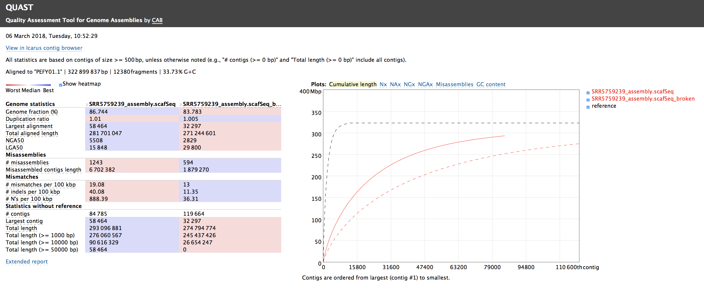
Figure 6.11: Screenshot of the report.html file showing the statistics and plots inferred by QUAST on the results of the SOAPdenovo2 assembly.
icarus.html: Icarus main menu with links to interactive viewers. Icarus generates contig size viewer and one or more contig alignment viewers (if reference genome is provided). All Icarus viewers contain a legend with color scheme description (see Figure 6.12).
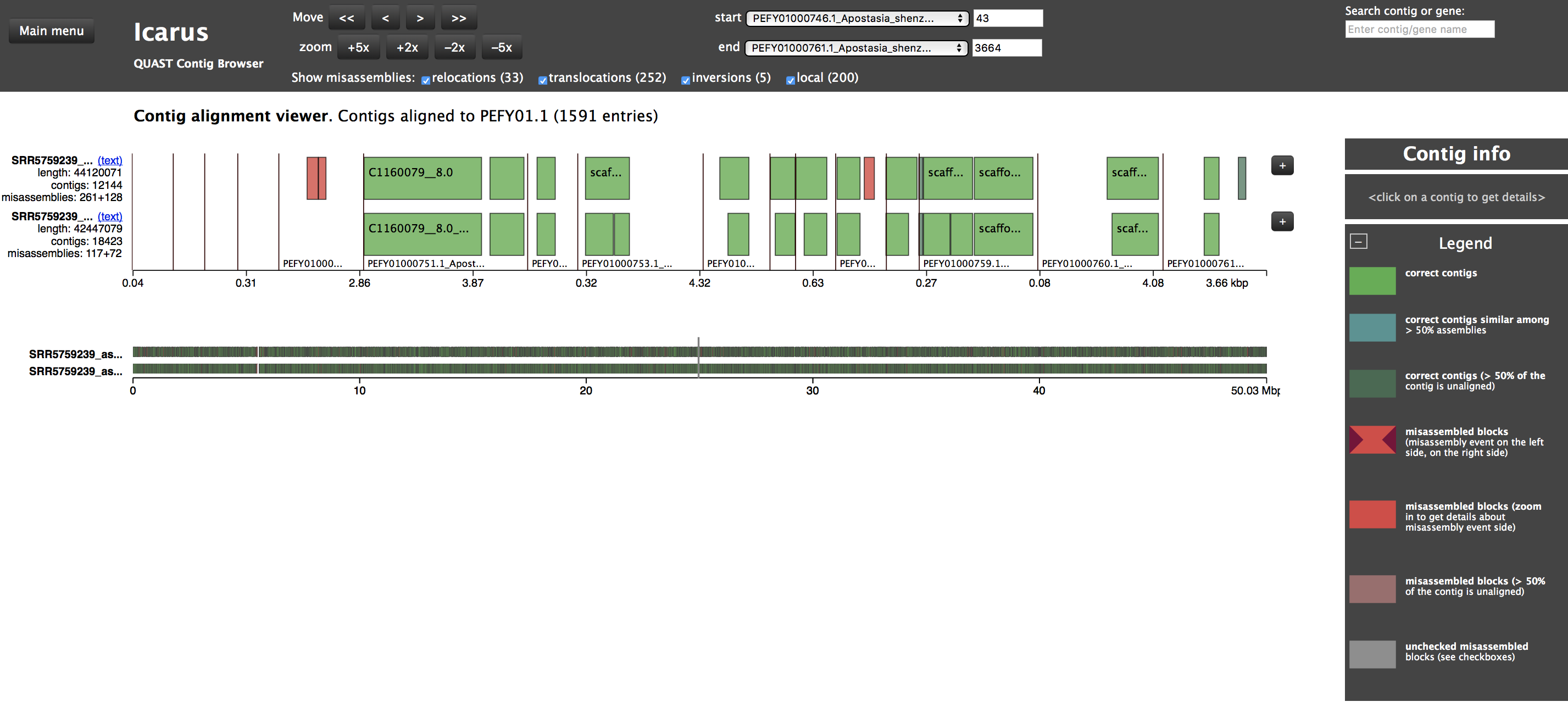
Figure 6.12: Screenshot of the icarus.html file showing the alignment of the SOAPdenovo2 de novo assembly against the reference genome.
6.10.5.1 Task and Questions
Do the following tasks:
- Transfer report.html on your computer.
- Inspect the statistics, plots and alignments (available by clicking on the
Icarustab; see Figure 6.11).
Questions
What is your overall assessment of the quality of the de novo assembly?
To reach your conclusion, ask yourself the following questions:
Did
SOAPdenovo2do a good job at assembling contigs into scaffolds?
What could be the implication(s) of using scaffolds to conduct gene annotation?