BIOL 497/597 - Genomics & Bioinformatics
Lab: Mining sagebrush draft genome
Sven Buerki - Boise State University
2026-04-24
1 Goal
The goal of this group lab report is to learn how to mine a draft genome to identify, extract, annotate, and validate a target protein-coding gene using bioinformatics tools. Through this investigation, you will gain practical experience working with genome assemblies and interpreting genomic data in a biological context, preparing you for genome-scale analyses in modern genomics.
2 Learning Outcomes
As part of this lab, students will learn how to mine a draft genome to identify, extract, annotate, and validate a target protein-coding gene, and interpret their findings in a biological context. Specifically, students will:
- Identify and extract target gene sequences from a draft Illumina genome assembly, applying genome mining approaches to locate coding regions of interest.
- Predict and annotate gene structure, including coding regions and gene features, to generate biologically meaningful gene models.
- Reconstruct protein sequences from annotated genes and interpret their structural and functional characteristics.
- Validate gene identity and infer protein function by comparing reconstructed sequences with reference databases and evaluating the strength of the evidence.
- Learn how to remotely access and work on a Unix-based computing environment to support genome mining analyses (see Tutorials).
- Use Unix and
Rtools to organize data, execute analyses, and support the extraction, annotation, and validation of genes (see Tutorials and Mini-Report 3).
3 Publication
This lab report is primarily based on the following publication:
- Melton et al. (2021) — A draft genome provides hypotheses on drought tolerance in a keystone plant species in Western North America threatened by climate change
- Online publication: https://doi.org/10.1002/ece3.8245
Additional references are provided throughout each section to help you master the material covered in this assignment.
4 Lab Report Workflow: Genome Mining, Gene Annotation, and Validation
This lab report guides you through a research-style investigation that integrates scientific reasoning with hands-on bioinformatics analyses. You will work with a draft genome to identify, extract, annotate, and validate aquaporin (AQP) genes, and interpret your findings in a biological context.
The assignment is organized into the following sections:
Group Activity 1: Investigating a Draft Genome Study and Its Genomic Resources You will collaboratively read and discuss the publication that forms the foundation of this lab report. This activity introduces the biological background, research question, and genomic resources generated in the study.
Group Activity 2: “Where’s Waldo?” – Designing a Genome Mining Strategy Building on the first activity, you will develop the theoretical framework needed to identify aquaporin genes in a draft genome. Using the Waldo analogy, you will define the key features of AQPs and design a bioinformatics strategy to locate them in genomic data.
Remote Computing and Bash Tutorials This section introduces the core computational tools used in this lab, including remote access (
ssh), job management (tmux), and Bash command-line workflows.Introduction This section presents the key concepts needed for the report, including the scientific question, hypothesis (and predictions), methodology, data availability, and report structure. Use this section as a reference throughout your analyses and writing.
Objectives and Scientific Question This section defines the specific objectives and research question you will investigate in this assignment.
Bioinformatics Analyses In this section, you will perform the analytical steps required to mine a draft genome and characterize aquaporin genes.
The analyses are structured in two stages:
- First, you will work collaboratively on a shared dataset to build the theoretical understanding and practical skills required for genome mining, gene annotation, and validation.
- Then, each group will be assigned a specific scaffold, which you will independently analyze to identify, annotate, and characterize your aquaporin gene. These hands-on modules connect theory to real genomic data and progressively build your confidence in applying bioinformatics workflows.
- Data Structure and Workflow: Overview of the dataset and project organization
- Module 1: Set up your working environment and identify scaffolds containing AQP genes
- Module 2: Extract candidate scaffolds and identify Open Reading Frames (ORFs)
- Module 3: Annotate ORFs and reconstruct AQP protein sequence(s)
- Module 4: Validate AQP protein sequences and infer their function(s)
- Data Interpretation: Guidance for interpreting results and preparing for downstream activities
- Your Turn: Apply the workflow to your assigned scaffold and interpret your results
Group Lab Report Detailed guidelines for writing and organizing your group lab report.
Group Lab Oral Presentation Guidelines for preparing and delivering your group presentation.
Evaluation Rubrics Criteria used to assess your lab report and oral presentation.
5 🤝 Group Activity 1: Investigating a Draft Genome Study and Its Genomic Resources
5.1 🧬 Learning Outcomes
By the end of this activity, you will be able to:
- Explain the scientific question addressed in a draft genome publication
- Describe how researchers generate, assemble, and analyze draft genome data
- Locate genomic datasets associated with a publication using NCBI databases
- Interpret how draft genome assemblies are used to investigate biological questions
- Prepare to mine and analyze a draft genome as part of your Group Lab Report
5.2 Activity Overview
In this 1 hour and 40 minute group activity, you will work in groups of 3–4 students to investigate the publication that forms the foundation of your Group Lab Report: Melton et al. (2021)
Through this activity, you will:
- Explore the biological motivation and research question of the study
- Examine how the draft genome was generated and analyzed
- Locate and investigate the associated genomic datasets on NCBI
- Prepare to use and mine this genome yourselves in the upcoming lab analyses
This activity will help you understand how genomic datasets are generated, organized, and shared in public repositories. It will also prepare you to navigate these resources and apply similar approaches when mining the draft genome analyzed in your Group Lab Report.
5.3 Materials
- Melton et al. (2021) — Draft genome publication
- NCBI — National Center for Biotechnology Information (genomic databases and tools)
- Genomic resources associated with the study on NCBI:
- BioProject — umbrella record describing the overall sequencing project
https://www.ncbi.nlm.nih.gov/bioproject/722258 https://www.ncbi.nlm.nih.gov/datasets/genome/GCA_021014915.1/ - Sequence Read Archive (SRA) — raw sequencing reads generated for the project
https://www.ncbi.nlm.nih.gov/sra?linkname=bioproject_sra_all&from_uid=722258
- Genome Assembly — assembled draft genome produced from the raw reads
https://www.ncbi.nlm.nih.gov/datasets/genome/GCA_023558565.1/
- BioProject — umbrella record describing the overall sequencing project
- Lexicon — reference definitions for key genomics and bioinformatics terms
5.4 Part 1 — What Biological Question Does This Study Address? (20 minutes)
As a group, read the Abstract and Introduction, then discuss:
- What organism is being studied?
- What makes this organism biologically or scientifically interesting?
- What is the main scientific question or objective of this study?
- Why is generating a draft genome important for answering this question?
- What types of downstream analyses do the authors intend to perform using this genome?
Group Outcome:
Write a brief summary (2–3 sentences):
What question does this study address, and why is a draft genome needed to answer it?
5.5 Part 2 — How Was the Draft Genome Generated and Used? (30 minutes)
Now read the relevant parts of the Methods and Results sections.
Discuss the following:
5.5.1 Genome sequencing
- What sequencing technology was used?
- Why is this technology appropriate for draft genome assembly?
5.5.2 Genome assembly
- What is a draft genome assembly?
- What information is provided about assembly quality (e.g., genome size, scaffold number)?
5.5.3 Genome mining and gene analysis
- What types of genes or genomic features do the authors investigate?
- Why are these genes important?
- How does the genome assembly allow the authors to extract and analyze these genes?
Group Outcome:
Explain in your own words:
How did the authors go from raw sequencing data to biological discoveries?
5.6 Part 3 — Locating the Raw Genomic Data on NCBI (25 minutes)
Goal: Learn how to locate and interpret genomic data associated with a published study.
You will use the Data Availability Statement of the publication to locate the genomic resources.
5.6.1 Identify accession numbers from the paper
Locate and record:
- BioProject accession number: ___________
- Raw sequencing reads accession number(s) (SRA): ___________
- Draft genome assembly accession number: ___________
5.6.2 Explore the BioProject
Go to:
Select BioProject and enter the accession number.
Discuss:
- What is the goal of this BioProject?
- What organism (referred to as BioSample in NCBI) is associated with it?
- What types of data are included?
5.6.3 Examine the raw sequencing reads
Locate the SRA data.
Discuss:
- How many sequencing runs are available?
- What sequencing platform was used?
- How much data was generated?
- Why are these raw reads important?
5.6.4 Examine the draft genome assembly
Locate the genome assembly record.
Discuss:
- What is the genome size?
- How many scaffolds does the assembly contain?
- What is the assembly level?
- Why is this called a draft genome?
5.6.5 Group Reflection
Discuss:
- Why is it important that these data are publicly available?
- How will you use this genome assembly in your lab project?
5.7 Part 4 — Connecting This Study to Your Lab Project (15 minutes)
Now think about your upcoming Lab Group Report.
Discuss:
- What types of genes will you be searching for in this genome?
- Why is genome mining possible only after genome assembly?
- What types of analyses will be required to:
- extract genes?
- annotate genes?
- validate gene identity and function?
Group Outcome:
Write:
What will you be able to discover by mining this genome?
5.8 Part 5 — Whole-Class Discussion (10 minutes)
We will conclude with a class discussion.
Each group will share:
- One key insight about the scientific goal of the study
- One important feature of the genome assembly
- One way the genome will be used in your lab project
5.9 Why This Activity Matters
This activity prepares you to:
- Work with real genomic data
- Understand how draft genomes are produced
- Locate and interpret genomic datasets
- Mine genomes to extract and analyze genes
These skills are essential for your Lab Group Report.
6 🤝 Group Activity 2: “Where’s Waldo?” – Designing a Genome Mining Strategy
6.1 🧬 Learning Objectives
By the end of this activity, you should be able to:
- Describe key structural and functional features of aquaporin proteins
- Distinguish major aquaporin subfamilies (e.g., PIP, TIP, NIP, SIP)
- Design a bioinformatics strategy to identify aquaporin genes in a draft genome
- Justify tool selection (e.g., BLAST, gene prediction, annotation)
- Recognize challenges associated with mining genes from draft assemblies
6.2 Activity Overview
In this 1 hour and 30 minute group activity, you will work in the groups assigned for this lab to develop a strategy for identifying aquaporin genes in a draft genome using a “Where’s Waldo?” analogy.
Just as finding Waldo requires knowing his defining features (striped shirt, glasses, hat), identifying genes in a genome requires understanding the diagnostic characteristics of the target gene family.
This activity is inspired by the study: Melton et al. (2021)
Through this activity, you will:
- Characterize the biological features of aquaporin proteins and their subfamilies (PIP, TIP, NIP, SIP)
- Identify the key “signature features” that distinguish aquaporins from other proteins
- Develop a bioinformatics strategy to locate aquaporin genes in a draft genome (FASTA format)
- Evaluate which tools (e.g., BLAST, gene prediction, annotation) are appropriate at each step
- Anticipate challenges associated with mining genes from draft genome assemblies
Rather than directly running analyses, you will focus on designing a logical and justified pipeline that you will later apply in your lab work.
This activity will prepare you to:
- Think critically about how genes are identified in unannotated genomes
- Understand how protein knowledge guides genome mining
- Apply similar strategies when working on your Group Lab Report
6.3 Materials
- Melton et al. (2021) — Aquaporin-focused draft genome study
- Course notes and Introduction section — Aquaporin structure, function, and subfamilies
- NCBI — for reference on sequence databases and BLAST tools
- Lexicon — reference definitions for key genomics and bioinformatics terms
6.4 🔍 Context: Where’s Waldo Meets Genomics (5 minutes)
Finding a gene in a genome is like finding Waldo in a crowded illustration.
To find Waldo, you need to know:
- What he looks like (striped shirt, glasses, hat)
- How he differs from others
- Where he is likely to appear
Similarly, to find aquaporin genes in a genome, you need to know:
- Their defining sequence and structural features
- How they differ from other membrane proteins
- What tools can detect those features in DNA sequences
👉 Goal: Develop a strategy to identify aquaporin genes from a draft genome assembly (FASTA format). This will be fundamental to conduct the bioinformatics analyses.
6.5 Part 1 – What Does “Waldo” Look Like? (30 minutes)
6.5.1 Task 1.1 – Protein Family Characteristics
Using:
- Melton et al. (2021)
- Your course notes
Answer:
- What is the main biological function of aquaporins?
- What type of protein are they (e.g., membrane, soluble)?
- What is their typical size (approximate amino acid length)?
6.5.2 Task 1.2 – Diagnostic Features
List at least 3 key features that define aquaporins:
- Structural features:
- Conserved motifs:
- Transmembrane domains:
💡 Hint: Think of these as “Waldo’s stripes and hat”.
6.5.3 Task 1.3 – Signature Motifs
- What are the NPA motifs?
- How many are typically present?
- Why are they important?
6.5.4 Task 1.4 – Subfamilies
Fill in the table:
| Subfamily | Full Name | Localization | Key Features |
|---|---|---|---|
| PIP | |||
| TIP | |||
| NIP | |||
| SIP |
6.5.5 Reflection
👉 What are the minimum features needed to confidently recognize an aquaporin?
6.6 Part 2 – Where to Look? (20 minutes)
You are given:
- A draft genome assembly (FASTA format)
- No annotation
6.6.1 Task 2.1 – The Challenge
Discuss:
- Why is it harder to find genes in a genome than in a protein database?
- What complications arise from draft assemblies?
6.6.2 Task 2.2 – Strategy Brainstorm
List possible approaches:
- Sequence similarity:
- Motif detection:
- Gene prediction:
👉 Which approach would you start with and why?
6.6.3 Task 2.3 – BLAST as a First Step
What type of BLAST would you use?
- BLASTn
- BLASTp
- tBLASTn
- BLASTn
Justify your answer.
What would you use as a query?
6.7 Part 3 – Building Your Strategy (25 minutes)
6.7.1 Task 3.1 – Step Ordering
Put the following steps in logical order:
- Identify candidate regions
- Extract genomic sequences
- Validate protein structure
- Perform BLAST search
- Annotate exon-intron structure
- Translate sequences
6.7.2 Task 3.2 – Fill in the Pipeline
Complete the workflow:
- Start with: __________________________
- Then: _______________________________
- Then: _______________________________
- Then: _______________________________
- Final validation: ____________________
6.7.3 Task 3.3 – Validation Criteria
How will you confirm a candidate is truly an aquaporin?
List at least 4 criteria:
- Presence of:
- Sequence similarity threshold:
- Structural features:
- Length range:
6.8 Part 4 – Challenges and Limitations (10 minutes)
6.8.1 Task 4.1 – Potential Pitfalls
Identify at least 3 challenges:
- Fragmented genes
- Assembly errors
- False positives
6.8.2 Task 4.2 – Improving Confidence
What could you add?
- Transcriptome data?
- Phylogenetic analysis?
- Domain prediction tools?
6.9 🧠 Final Reflection (5 minutes)
In 2–3 sentences:
👉 How is finding aquaporins in a genome similar to finding Waldo?
👉 What makes bioinformatics both powerful and uncertain?
7 Introduction
This document supports analyses aiming at mining the sagebrush (Artemisia tridentata Nutt; Asteraceae) draft genome for Aquaporin (AQP) genes and it is based on data and analyses presented in Melton et al. (2021). AQPs are multi-exon genes (see Figure 7.1) encoding for a large family of proteins known to function in the transport of water and other molecules across cell membranes (reviewed in Li et al., 2014).
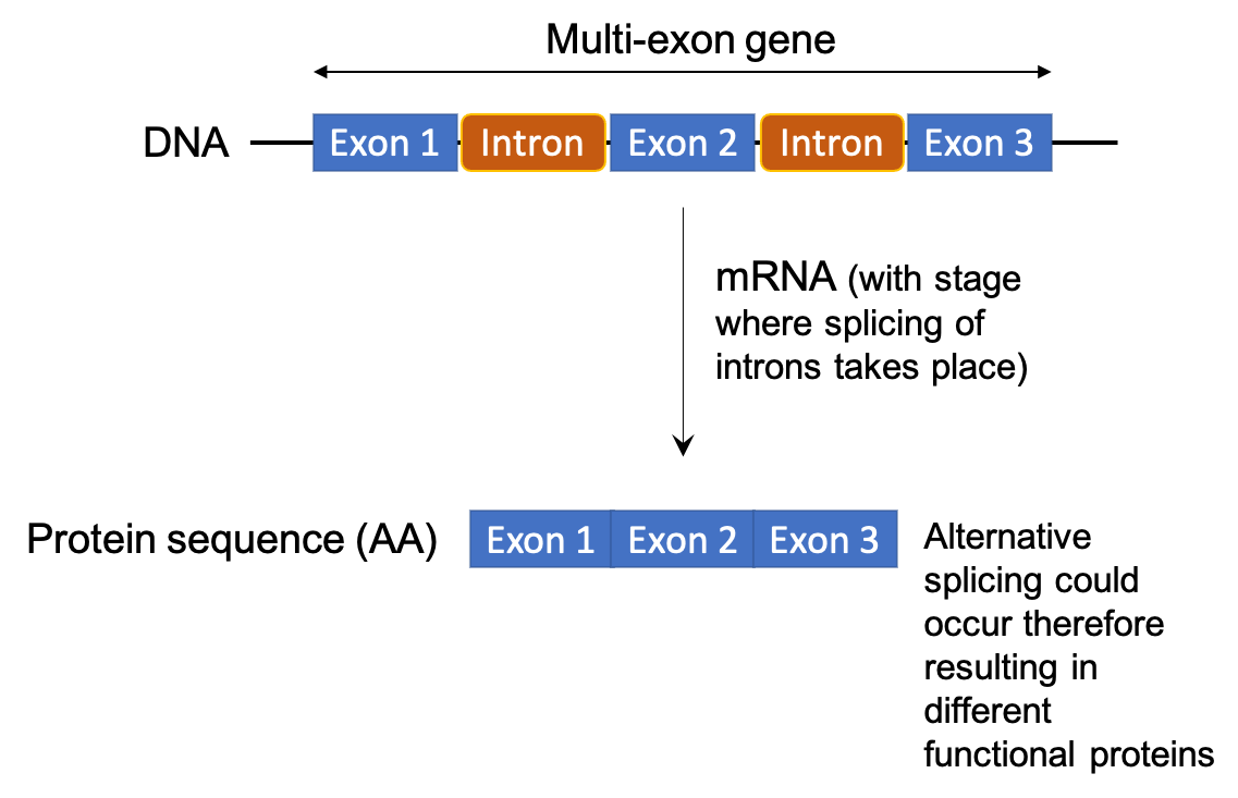
Figure 7.1: Flowchart showing the structure of a multi-exon gene and different resulting proteins. As a reminder, exons are pieces of coding DNA that encode proteins. Different exons code for different domains of a protein. The domains may be encoded by a single exon or multiple exons spliced together. In the case of multi-exon genes, the presence of exons and introns allows for greater molecular evolution through the process of exon shuffling and alternative splicing. Exon shuffling occurs when exons on sister chromosomes are exchanged during recombination. This allows for the formation of new genes. On the other hand, exons also allow for multiple proteins to be translated from the same gene through alternative splicing. This process allows the exons to be arranged in different combinations when the introns are removed/spliced. The different configurations can include the complete removal of an exon, the inclusion of part of an exon, or the inclusion of part of an intron. Alternative splicing can occur in the same location to produce different variants of a gene with a similar role, such as the human slo gene, or it can occur in different cell or tissue types, such as the mouse alpha-amylase gene. Alternative splicing, and defects in alternative splicing, can result in a number of diseases including cancer.
7.1 AQP defining characteristics
The defining characteristics of AQP proteins include having:
- Six membrane-spanning alpha-helices
- Two hydrophobic loops
- Each loop contains a conserved asparagine-proline-alanine (NPA) motif forming a barrel surrounding a central pore-like region that contains additional protein density (see Figure 7.2)
While the NPA motifs are generally highly conserved, there are some AQP genes that have undergone mutations of the alanine residue in the NPA motif (Ishibashi, 2006).
7.2 AQP subfamilies
AQPs in flowering plants comprise five subfamilies (Danielson and Johanson, 2008):
- NOD26-like intrinsic proteins (NIPs);
- plasma membrane intrinsic proteins (PIPs);
- small basic intrinsic proteins (SIPs);
- tonoplast intrinsic proteins (TIPs);
- X intrinsic proteins (XIPs).
Genes from each subfamily tend to move water or other substrate depending on their NPA motifs. Some AQPs, such as NIPs, have acquired a mutation in their NPA motif, such as alanine to leucine, which confer the ability to move substrates such as urea or ammonium (reviewed in Chaumont et al., 2005).
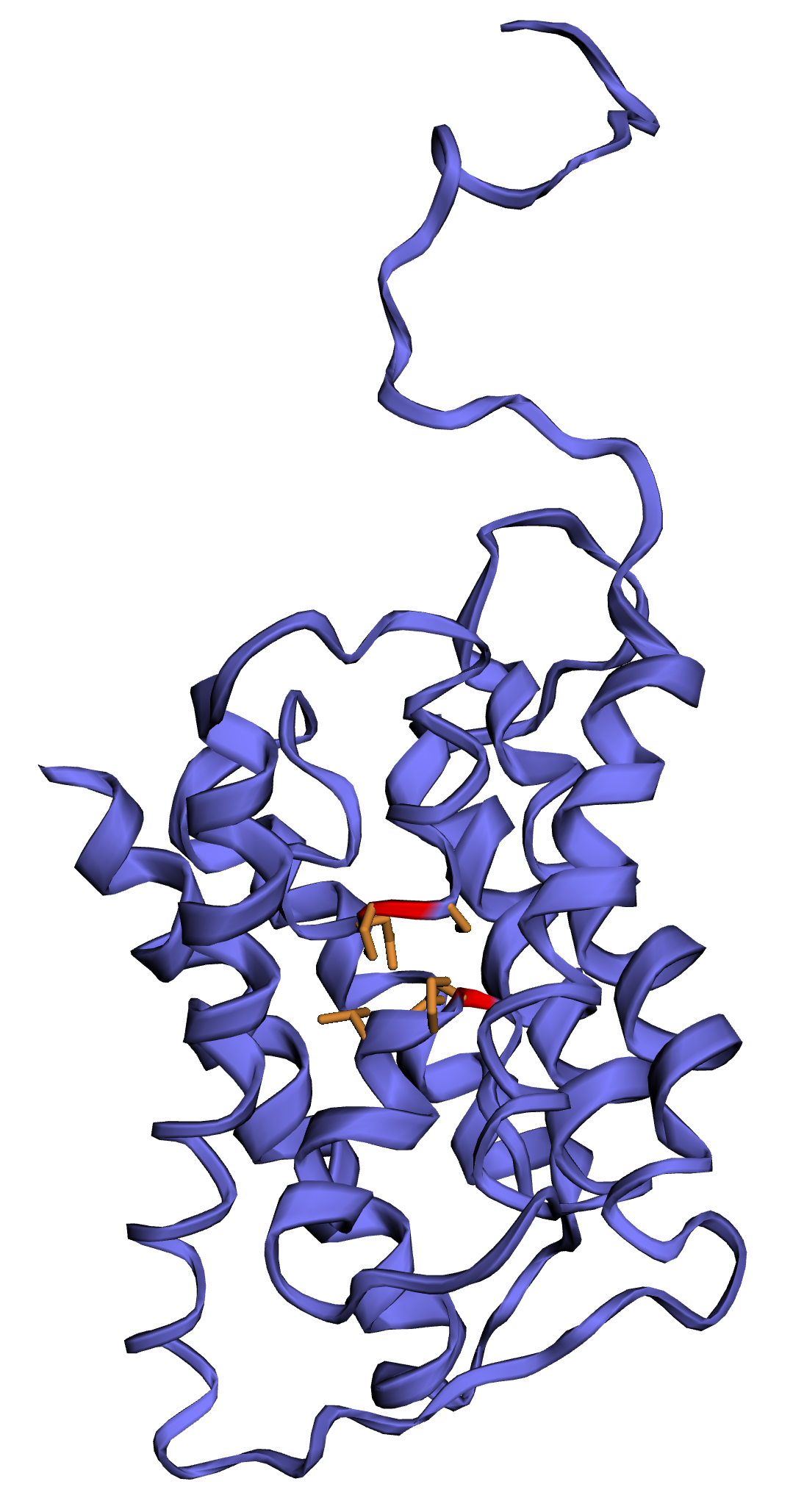
Figure 7.2: Example of a 3D model of an Aquaporin protein recovered in the sagebrush genome. NPA motifs are shown by red/orange colors
8 Objectives and Scientific Question
The instructor teaches students to conduct analyses by going over each module in class demonstrating the approach to mine genome for target gene and go over steps to assemble and validate protein product. Then, each group will be assigned a scaffold (from the de novo genome assembly) and they will have to conduct analyses presented in modules 2 to 4 on their own to answer the following question:
What Aquaporin protein coding sequence is “hidden” in your assigned scaffold?
Very much the same as with the “Where’s waldo?” children books, students will be able to make predictions to “find” their Aquaporin protein coding sequence based on material presented in the Introduction and further developed in modules 2, 3 and 4. These material will allow students to design their analytical workflow covering the following major steps:
- Predict, annotate and identify AQP genes along scaffold.
- Reconstruct and validate AQP protein sequences.
- Predict AQP protein function (by intersecting evidence recovered from the previous steps).
8.1 Scaffolds assigned to groups
The FASTA file with scaffolds sequences can be downloaded here. The scaffolds assigned to each group are as followed:
- Group 1: Scaffold106379.
- Group 2: Scaffold254734.
- Group 3: Scaffold348135.
Let’s complete the training first going by through each module and then students will be working in groups to replicate these analyses to their assigned scaffold.
9 Groups and Data Structure
9.1 Group Organization and Structure
Each group is composed of 5 to 6 students, with a mix of undergraduate and graduate students to promote peer learning and knowledge exchange.
Each group is divided into two subgroups (A and B). Both subgroups will perform the same analyses in parallel, working independently at first.
This structure is designed to:
- Encourage fact-checking by comparing results between subgroups
- Improve accuracy and reproducibility
- Build confidence in computational results through independent validation
9.2 Group Accounts
Each group has been assigned two accounts:
- One account for Subgroup A
- One account for Subgroup B
Each subgroup must use its assigned account to complete the exercises.
You will access the Linux systems using the ssh protocol. Details on your account information are available here.
9.3 Group Collaboration Guidelines
- Each subgroup works independently using its assigned account
- Analyses are conducted in parallel by Subgroup A and Subgroup B
- All accounts within a group share the same computational resources
- Coordinate within your subgroup to avoid conflicts when running intensive jobs
- After completing tasks, compare results between subgroups to verify accuracy
- Discuss and resolve any discrepancies before moving forward
9.3.1 Technical Notes
- All accounts use the same password for simplicity
- Accounts have access to the bioinformatics software required for the course
- File permissions allow collaboration within each account environment
- Contact the instructor if you experience connection issues
9.4 Where are the data located?
All data associated with this project are located in your account in the DraftGenomeMineR/ directory:
~/DraftGenomeMineRKey files:
Draft_Genome_Assembly.fasta: Sagebrush draft genome assembly (scaffold level)FASTAs/PIP1_3.fa: Reference file containing the PIP1 protein sequence for BLAST analysisLesson_Modules/: Scripts associated with each module
10 Module 1
10.1 Objectives
This module is dedicated to presenting approach to set-up your working environment and then to identify scaffolds in the de novo genome assembly containing AQP genes (using BLAST).
10.2 Remotely connect to computer
Start by using ssh protocol to connect to your Linux computer. This is done as follows (enter password when prompted to):
#SSH with bio_11 as example
ssh bio_11@132.178.142.214
10.3 Install R v.4.1.3
!!WARNING: YOU DON’T HAVE TO INSTALL R!!
The code used in this lab depends on a specific version of R (version 4.1.3 (2022-03-10) – “One Push-Up”) and it needs to be installed on your computer prior to starting the tutorial. This can be done by following the procedure described on these two websites:
http://genomespot.blogspot.com/2020/06/installing-r-40-on-ubuntu-1804.html
https://www.digitalocean.com/community/tutorials/how-to-install-r-on-ubuntu-18-04
Disclaimer: The right version of R was already installed on our lab computers, but if you wanted to execute this code on your personal computer please make sure you have the right version of R!
10.4 Start R session and associated R script
10.4.1 To do before starting
Before starting this tutorial, do the following:
- Remotely connect to your computer
- Start a new
tmuxsession entitled “Lab” on your remote computer - Navigate to
DraftGenomeMineR/and start a newRsession:
#Navigate to DraftGenomeMineR/
cd DraftGenomeMineR/

#Start R session
R- Create and save a new R file in RStudio entitled
Lab_mining_genome.Ron your personal computer
10.5 R dependencies
!!! DON’T EXECUTE THIS CODE !! The instructor already installed the R packages on your computers, but the code below shows you how these packages were installed.
Some of the required packages cannot be installed with install.packages() and require the BiocManager R package to be installed. We are also installing some packing directly from GitHub repositories.
#Check if BiocManager is installed and if not install it
if (!require("BiocManager", quietly = TRUE))
    install.packages("BiocManager")
BiocManager::install()

#Install the other packages using BiocManager
install.packages("devtools")

library(devtools)
BiocManager::install("Biostrings")
BiocManager::install("ORFik")

#Install required packages for this tutorial
install_github("mhahsler/rBLAST")
install.packages("remotes")
remotes::install_github("GuillemSalazar/FastaUtils")
install.packages("ape")
install.packages("seqinr")
10.6 Load R packages and user-defined functions
To conduct the analyses, you need to load R packages and source R user-defined functions. Please copy the following code in your R script and then execute it.
10.6.1 Bioinformatics
- Create an object with all the required R packages and load them:
# This will make a list of packages that another function will use to make sure they are all installed and loaded.
list.of.packages <- c("ape",
                      "Biostrings",
                      "dplyr",
                      "FastaUtils",
                      "ORFik",
                      "readr",
                      "tidyr",
                      "rBLAST",
                      "seqinr",
                      "stringr")

# Use lapply to load all of the packages in the list.
lapply(list.of.packages, require, character.only = TRUE)- Load all the user-defined function located in
Functions/:
# Load all of the functions written for DraftGenomeMineR
files.sources <- list.files("Functions", full.names=T)
sapply(files.sources, source)
10.7 Set environment for BLAST analysis
To be able to navigate between folders within our project, we will set an object entitled project.folder, which contains the path to the root of the project folder.
10.7.1 Bioinformatics
To create this object, do as follows:
- Create an object with working directory
#Copy the output of getwd() in the object as follows:
project.folder <- getwd()
Call project.folder in the Console to check that it is correct. It should return:
"~/DraftGenomeMineR".
- Set working directory to
project.folderas follows:
#Set working directory
setwd(project.folder)
10.8 Run the BLAST analysis
10.8.1 Overview
In this section, you will perform a BLAST analysis to identify scaffolds containing AQP genes. For this analysis, you will need the following files:
- Input:
Draft_Genome_Assembly.fasta: The file containing all the scaffolds (= draft genome)FASTAs/PIP1_3.fa: The file containing an AQP protein sequence used to mine the draft genome
- Output:
Unique_Filtered_Blast_Hit_Info.csv: A CSV containing the results of the BLAST analysis (= which scaffold matches the AQP protein sequence)
10.8.2 Bioinformatics
- Set general parameters for the BLAST analysis:
# There are a few parameters that need to be set.
# Let's create some R objects to store file paths and parameters for the BLAST search.

# We need a query (a fasta file of a gene you want to find in the draft genome), a draft genome assembly, BLAST databases, paths to other required folders (described in the README), and other parameters that can be used to filter results.
query.file.path <- "FASTAs/PIP1_3.fa"
genome.file.name <- "Draft_Genome_Assembly.fasta"
genome.path <- "FASTAs/Draft_Genome_Assembly.fasta"
blast.db.path <- "BlastDBs/Draft_Genome_Assembly.fasta"
AA.BlastDB.folder <- "AA_BlastDB/"
AA.ORF.folder <- "AA_ORFs/"
max.e <- 5E-50
perc.ident <- 90.000
query.type <- "AA"
blast.type <- "tblastn"
make.BlastDB <- T
BlastDB.type <- "nucl"- Read in the sagebrush draft genome assembly in
FASTAformat:
# Read in the genome assembly file
genome <- readLines(con = genome.path)
head(genome) # Print the top 6 lines of the fasta. There should be no spaces in what is printed. Each header should be on one line, followed by its entire scaffold on the next.- Make a BLAST database for query:
# Do you need to make a BLAST database or use an existing one?
if(make.BlastDB == TRUE){
  setwd("BlastDBs/")
  makeblastdb(file = genome.file.name, dbtype = BlastDB.type)
}- Read in the query file in
FASTAformat:
# Read in the query. What type of molecule is the query? DNA (or RNA) or amino acid sequences?
setwd(project.folder) # Previous lines changed the wd, so we need to go back to the project folder.
if (query.type == "DNA") {
  query <- readDNAStringSet(filepath = query.file.path,
                            format = "fasta")
} else {
  query <- readAAStringSet(filepath = query.file.path,
                           format = "fasta")
}- Perform BLAST analysis (
BLASTneeds to be installed on the computer):
# Now we have everything set up and can perform a BLAST search.
bl <- blast(db = blast.db.path, type = blast.type) # Create an object with the BLAST database and the type of BLAST search to perform.
cl <- predict(bl, query) # Perform the BLAST search
head(cl) # Look at the top BLAST hits- Filter output of BLAST analysis:
# We can now filter out bad BLAST hits using a few thresholds and parameters. This leaves us with only the best matches to our query.
# What parameters do you think would give you just the best candidates to be your gene of interest?
cl.filt <- subset(x = cl, Perc.Ident >= perc.ident & E <= max.e)
cl.filt.unique <- cl.filt[!duplicated(cl.filt[,c('SubjectID')]),] # SubjectID is the column that contains the scaffold names
cl.filt.unique
nrow(cl)
nrow(cl.filt)
nrow(cl.filt.unique)
blast.hits.to.extract <- subset(x = cl.filt.unique, SubjectID == cl.filt.unique[1,2])- Write output of BLAST analysis in
csvfile:
# We have evaluated the top BLAST hits and can see a clear best hit. Let's save this data so we can extract just that scaffold later.
write.csv(x = blast.hits.to.extract, file = "Unique_Filtered_Blast_Hit_Info.csv", row.names = F)- Quit R (using quit()) and inspect the content of
Unique_Filtered_Blast_Hit_Info.csvusing e.g.vim.
11 Module 2
11.1 Objectives
In this module, we are conducting the following tasks:
- Setting up your working environment (as shown in module 1)
- Extracting scaffold(s) identified in module 1 from the de novo draft genome assembly (in
FASTAs/Draft_Genome_Assembly.fasta) and saving the output as aFASTAobject/file. - Finding ORFs along scaffold(s) using the user-defined function findORFsTranslateDNA2AA() and saving the output into a
FASTAobject/file. In molecular genetics, an Open Reading Frame (ORF) is the part of a reading frame that has the ability to be translated. An ORF is a continuous stretch of codons that begins with a start codon (usually AUG) and ends at a stop codon (usually UAA, UAG or UGA). We will study the code implemented in findORFsTranslateDNA2AA() to fully understand the applied approach. - Produce maps of recovered ORFs along scaffold(s). These
pdfmaps will be saved inORFs_map/.
11.2 Setting up your working environment
Before starting analyses in R, students have to complete these following tasks:
- Remotely connect to their computers (using their individual accounts) with
sshprotocol. - Navigate to project directory (
DraftGenomeMineR/) usingcd. - Create a new folder (
Output_FASTAs/) usingmkdirto store results of BLAST scaffold analysis. - Create a new folder (
ORFs_report/) usingmkdirto store results of ORFs analysis. - Start a new
Rsession usingR-4command. - Load R packages and user-defined functions.
- Set working directory to
DraftGenomeMineR/.
For an example of code, see below:
#1. ssh
ssh svenbuerki@132.178.142.214

#2. Navigate to DraftGenomeMineR/
cd DraftGenomeMineR/

#3. & 4. Create new folders to save files
# --> If these folders already exist then don't execute the following code
mkdir Output_FASTAs/
mkdir ORFs_report/

#5. Start R session
R

#6. This will make a list of packages that another function will use to make sure they are all installed and loaded.
list.of.packages <- c("ape",
                      "Biostrings",
                      "dplyr",
                      "FastaUtils",
                      "ORFik",
                      "readr",
                      "tidyr",
                      "rBLAST",
                      "seqinr",
                      "stringr")

# Use lapply to load all of the packages in the list.
lapply(list.of.packages, require, character.only = TRUE)

# Load all of the functions written for DraftGenomeMineR
files.sources <- list.files("Functions", full.names=T)
sapply(files.sources, source)

#7. Copy the output of getwd() in the object as follows:
project.folder <- getwd()

#Set wd
setwd(project.folder)
11.3 Extract scaffold(s) in draft genome
11.3.1 Overview
In this section, you will use the output of the BLAST analysis to extract the scaffold containing the AQP gene. For this analysis, you will need the following files:
- Input:
FASTAs/Draft_Genome_Assembly.fasta: The file containing all the scaffolds (= draft genome)Unique_Filtered_Blast_Hit_Info.csv: A CSV containing the results of the BLAST analysis (= which scaffold matches the AQP protein sequence)
- Output:
Output_FASTAs/Scaffold151535.fa: A FASTA file with the scaffold containing the AQP gene
!!NOTE: Don’t forget to copy paste the code in your R script!!
11.3.2 Bioinformatics
- In
R, openUnique_Filtered_Blast_Hit_Info.csvcontaining results of BLAST analysis and extract name of target scaffold(s)
#Open BLAST file
cl.filt.unique <- read.csv(file = "Unique_Filtered_Blast_Hit_Info.csv") # Output of module 1

#Scaffold IDs
cl.filt.unique$SubjectID- Extract scaffold(s) sequences from draft genome file (
FASTAs/Draft_Genome_Assembly.fasta)
#Open draft genome file
genome <- readLines("FASTAs/Draft_Genome_Assembly.fasta")

#Check formatting of file
head(genome)

#How many scaffolds?
Nscaff <- length(genome)/2

#Extract scaffolds in a loop

#Create data frame to store scaffold data
scaffold <- data.frame("scaffoldID" = character(length(cl.filt.unique$SubjectID)), "scaffoldSeq" = character(length(cl.filt.unique$SubjectID)))
#Start populating data frame
scaffold$scaffoldID <- cl.filt.unique$SubjectID

for(i in 1:nrow(scaffold)){
  # Find and Extract seq of each scaffold from draft genome FASTA file
  scaffold$scaffoldSeq[i] <- genome[match(paste0(">",scaffold$scaffoldID[i]), genome)+1]
}

#Convert into FASTA format
scaffoldFASTA <- apply(scaffold, 1, paste, collapse="\n")

#Save/export FASTA file
write.table(scaffoldFASTA, "Output_FASTAs/Scaffold151535.fa", row.names = F, col.names=F, quote = F)
11.4 Find ORFs along scaffold(s)
11.4.1 Overview
In this section, you will find ORFs along the scaffold containing the AQP gene. For this analysis, you will need the following files:
- Input:
Output_FASTAs/Scaffold151535.fa: A FASTA file with the scaffold containing the AQP gene
- Output:
ORFs_report/Scaffold151535_ORFs.csv: A CSV file with all predicted ORFs along scaffoldAA_ORFs/Scaffold151535_ORFs.fa: A FASTA file with AA sequences for all predicted ORFs (= input for module 3)ORFs_map/Scaffold151535_ORFs_annotated.pdf: A PDF with the map of all recovered ORFs along the scaffold
!!NOTE: Don’t forget to copy paste the code in your R script!!
11.4.2 Bioinformatics
We will now find ORFs in scaffold(s) using findORFsTranslateDNA2AA(). This user-defined function (UDF) relies on functions from the ORFik R package. The output will be saved in ORFs_report/.
Let’s first look at the structure of the findORFsTranslateDNA2AA() function to understand the applied approach:
##################################
#WARNING: DON'T EXECUTE THIS CODE#
##################################

#####~~~
#A UDF used to findORFs in scaffold file (FASTA format) and produce AA sequences as well as report
#####~~~
findORFsTranslateDNA2AA <- function(scaffold, scaffoldID, MinLen){
  #Extract scaffold sequence (and convert to right format)
  seqRaw <- scaffold[c(grep(paste(">", scaffoldID, sep=''), scaffold)+1)]
  seqs <- DNAStringSet(seqRaw)

  #positive strands
  pos <- ORFik::findORFs(seqs, startCodon = "ATG", minimumLength = MinLen)

  #negative strands (DNAStringSet only if character)
  neg <- ORFik::findORFs(reverseComplement(DNAStringSet(seqs)), startCodon = "ATG", minimumLength = MinLen)
  pos <- relist(c(GRanges(pos,strand = "+"),GRanges(neg,strand = "-")),skeleton = merge(pos,neg))

  #Process output
  pos <- as.data.frame(pos)
  pos$scaffoldID <- rep(scaffoldID, nrow(pos))
  pos$ORFID <- paste("ORF_", seq(from=1, to=nrow(pos)), sep='')

  #Extract and write ORFs from seq and produce AA sequence
  for(i in 1:nrow(pos)){
    if(as.character(pos$strand[i]) == "+"){
      extSeq <- as.DNAbin(DNAStringSet(paste(strsplit(seqRaw, split='')[[1]][c(pos$start[i]:pos$end[i])], collapse = "")))
      AAseq <- paste(paste(">", pos$scaffoldID[i], "_", pos$ORFID[i], sep=''), paste(as.character(trans(extSeq, code = 1, codonstart = 1))[[1]], collapse = ''), sep='\n')
      write.table(AAseq, file = paste("AA_ORFs/", pos$scaffoldID[i], "_", pos$ORFID[i], ".fa", sep=''), col.names = F, row.names = F, quote = F)
    }
    if(as.character(pos$strand[i]) == "-"){
      revComp <- reverseComplement(DNAStringSet(seqs))

      extSeq <- as.DNAbin(DNAStringSet(paste(strsplit(as.vector(revComp), split='')[[1]][c(pos$start[i]:pos$end[i])], collapse = "")))
      AAseq <- paste(paste(">", pos$scaffoldID[i], "_", pos$ORFID[i], sep=''), paste(as.character(trans(extSeq, code = 1, codonstart = 1))[[1]], collapse = ''), sep='\n')
      write.table(AAseq, file = paste("AA_ORFs/", pos$scaffoldID[i], "_", pos$ORFID[i], ".fa", sep=''), col.names = F, row.names = F, quote = F)
    }
  }

  #Merge all ORFs for BLAST analysis
  system(paste("cat AA_ORFs/", pos$scaffoldID[i], "* > AA_ORFs/", pos$scaffoldID[i], "_ORFs.fa", sep=''))
  system(paste("rm AA_ORFs/", pos$scaffoldID[i], "_ORF_*", sep=""))
  #Save pos file
  write.csv(pos, file = paste("ORFs_report/",pos$scaffoldID[i], "_", "ORFs.csv", sep=''), col.names = T, row.names = F, quote = F)
} - Now, we can apply findORFsTranslateDNA2AA() to our data:
# Open FASTA file with target scaffold
scaffold <- readLines("Output_FASTAs/Scaffold151535.fa")
scaffoldID <- grep(pattern = "^>", x = scaffold, value = T)
scaffoldID <- gsub(pattern = ">", replacement = "", x = scaffoldID)
# Apply UDF to find ORFs and translate these into AA
# --> we will use the AA sequences to conduct a BLAST analysis and identify ORFs coding for Aquaporin exons
tryCatch(
  {
    for(i in 1:length(scaffoldID)){
      findORFsTranslateDNA2AA(scaffold = scaffold, scaffoldID = scaffoldID[i], MinLen = 40)
    }
})- We should now have ORFs reports and
FASTAfiles of translated ORFs. Let’s check these outputs.
# Open the CSV output of the UDF containing data on predicted ORFs and associated sequences
orf.report <- read.csv("ORFs_report/Scaffold151535_ORFs.csv")

# How many ORFs were found?
nrow(orf.report)

# What are the longest ORFs?
orf.report[order(-orf.report$width),]

# Look at translated ORFs (=AA sequences)
translated.orfs <- readLines("AA_ORFs/Scaffold151535_ORFs.fa")
head(translated.orfs)
11.5 Produce maps of recovered ORFs along scaffold(s)
Here, we are visualizing the ORFs recovered by our analysis along each scaffold by producing maps saved in pdf format in ORFs_map/. The code also checks if the folder ORFs_map/ where files will be saved exists and if not creates it.
11.5.1 Bioinformatics
First study the code provided below and then execute it. Don’t forget to copy and paste it in your R script.
###
#Build map of scaffold with ORFs
###

#Read scaffold FASTA file (line by line)
scaffold <- readLines("Output_FASTAs/Scaffold151535.fa")

#List all files with ORFs
ORFfiles <- list.files(path = "ORFs_report", pattern = ".csv", full.names = T)

#Check if folder where ORF maps will be saved exists
# if not then creates it
output_dir <- file.path(paste0(getwd(), "/ORFs_map/"))

if(dir.exists(output_dir)){
  print(paste0("Dir", output_dir, " already exists!"))
}else{
  print(paste0("Created ", output_dir))
  dir.create(output_dir)
}

#Produce a map (in pdf format) for each scaffold
for(i in 1:length(ORFfiles)){
  print(ORFfiles[i])
  #Read file in
  ORF <- read.csv(ORFfiles[i])

  #Process FASTA scaffold sequence
  seq <- strsplit(scaffold[grep(paste(">", ORF$scaffoldID[1], sep=''), scaffold)+1], split='')

  #Separate ORFs by strand
  ORFplus <- subset(ORF, ORF$strand == "+")
  ORFneg <- subset(ORF, ORF$strand == "-")

  #Create plot
  pdf(paste("ORFs_map/", ORF$scaffoldID[1], "_ORFs_annotated.pdf", sep=''))

  #Initiate plot
  plot(x=1, y=1, xlim=c(0,length(seq[[1]])), ylim=c(0,2), type='n', bty="n", axes=F, xlab = "", ylab='')
  #Add title
  text(x=5, y=2, paste(ORF$scaffoldID[1], " (strand: + in grey and - in blue)", sep=''), adj=0, cex=.8)

  #Create a segment with length of scaffold
  segments(x0=0, x1=length(seq[[1]]), y0=1, y1=1, col='black', lwd=3)

  #Add ORFs: rectangles (grey: +, blue: -)
  rect(xleft=ORFplus$start, xright=ORFplus$end, ybottom=0.75, ytop=1.25, col='grey')
  rect(xleft=ORFneg$start, xright=ORFneg$end, ybottom=0.75, ytop=1.25, col='blue')
  text(x=(ORFneg$start + ORFneg$end)/2, y=0.7, paste(ORFneg$ORFID, " (", ORFneg$start, ":", ORFneg$end, ")", sep=''), srt=90, col='blue', adj=1, cex=0.4)
  text(x=(ORFplus$start + ORFplus$end)/2, y=1.3, paste(ORFplus$ORFID, " (", ORFplus$start, ":", ORFplus$end, ")", sep=''), srt=90, col='black', adj=0, cex=0.4)

  #Add x axis
  axis(side = 1)
  mtext("Sequence (bp)", pos = c(0,0.5), side=1, line=2, cex.lab=0.6,las=1)
  #Close pdf
  dev.off()
}
Figure 11.1 shows the location of the predicted ORFs along Scaffold151535 inferred by the code displayed above.
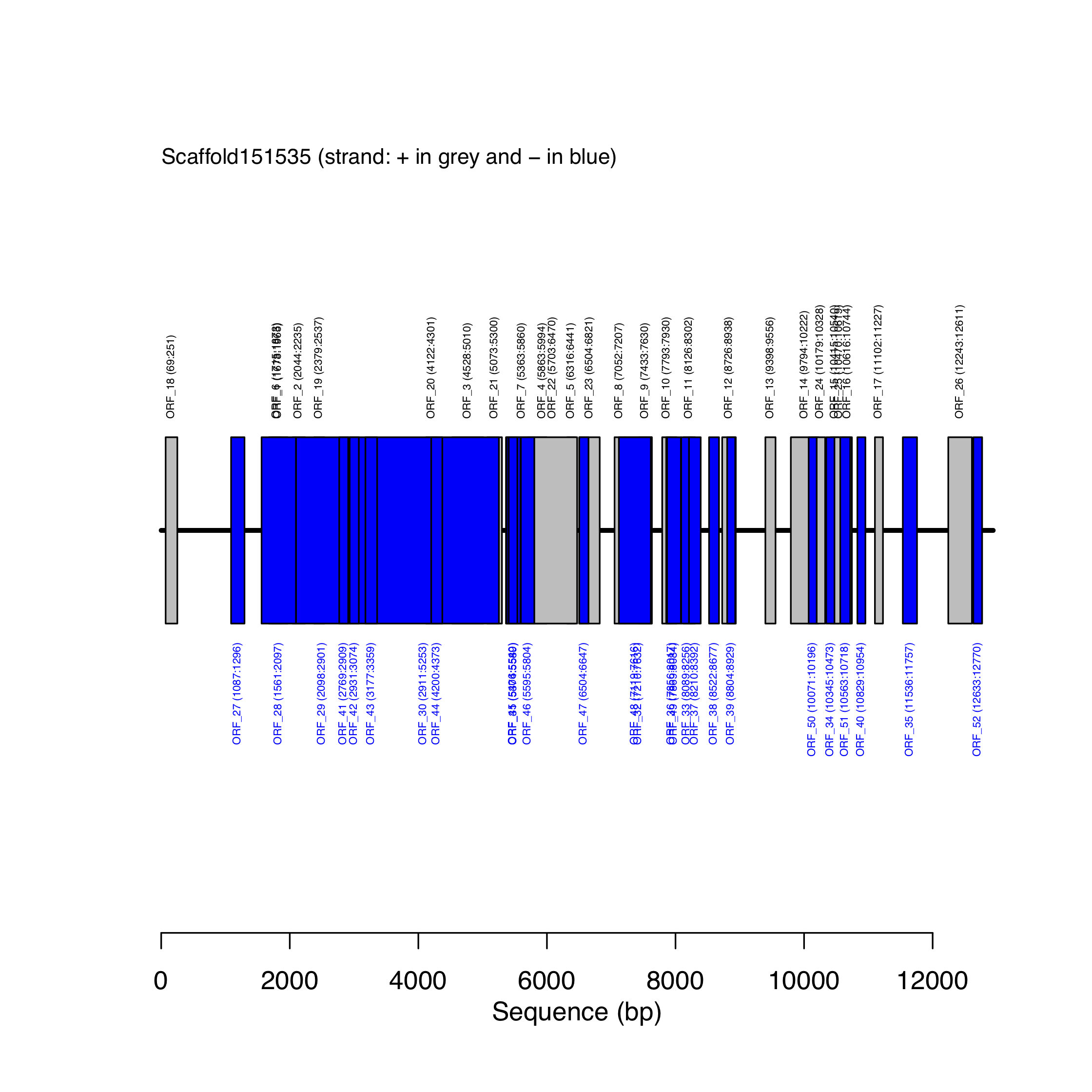
Figure 11.1: Map of predicted ORFs along scaffold151535.
11.6 Questions
How many ORFs were discovered on
Scaffold151535?
How many ORFs are on the
+and-strands?
Write an R code based on ORFs_report/Scaffold151535_ORFs.csv to answer the questions.
12 Module 3
12.1 Objectives
In this module, we are conducting the following tasks:
- Annotate ORFs inferred in module 2 using online protein BLAST tool. Students will use the output of the protein BLAST analysis to identify ORF(s) coding for Aquaporin genes.
- Extract ORF(s) identified by protein BLAST analysis to reconstruct Aquaporin gene sequence. Students will provide DNA sequence of Aquaporin gene located on scaffold and its associated protein sequence.
12.2 Annotate ORFs using online protein BLAST tool
12.2.1 Input file for protein BLAST analysis
The FASTA file Scaffold151535_ORFs.fa (see Figure 12.1) contains amino acid (AA) sequences of open reading frames (ORFs) identified in Module 2.
This file is located in the directory ~/DraftGenomeMineR/AA_ORFs. It can also be downloaded from the shared Google Drive or from GitHub.
Alternatively, you can use FileZilla to transfer the file from your Linux machine to your local computer.
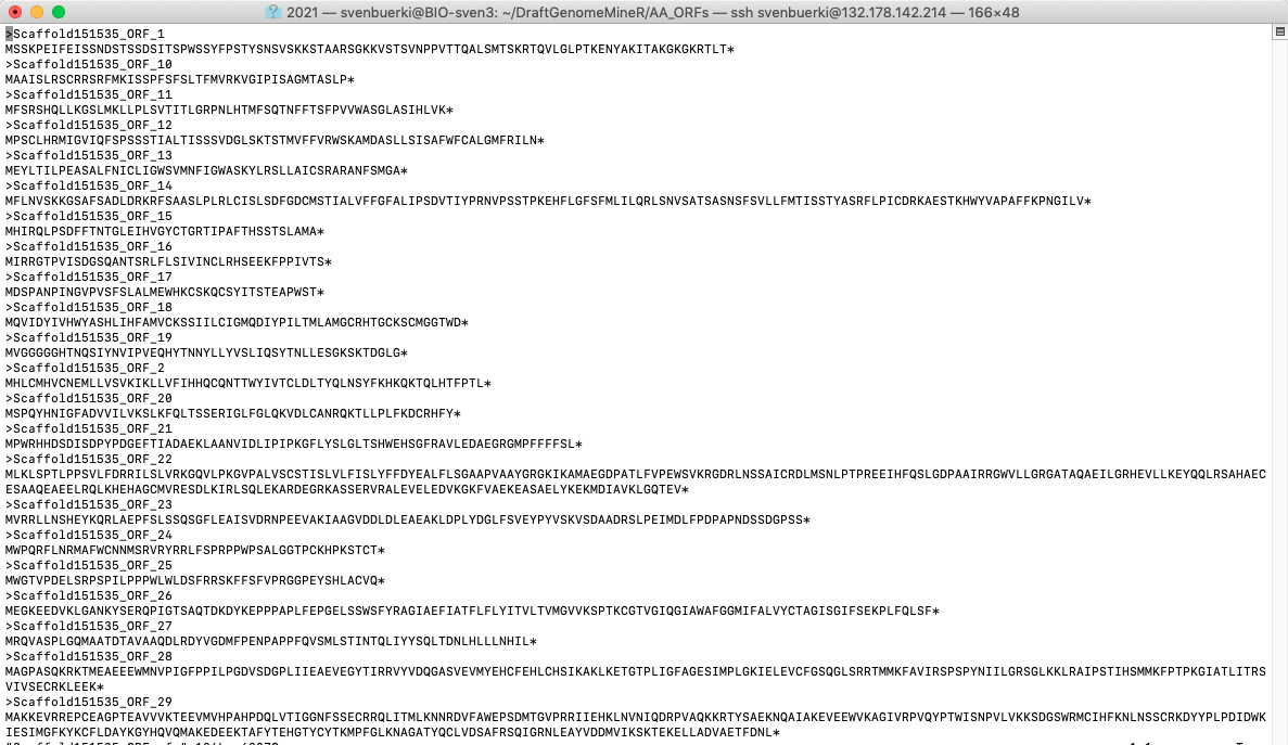
Figure 12.1: FASTA file containing all AA sequences for ORFs inferred along scaffold. See module 2 for more details.
12.2.2 Protein BLAST analysis
- Students download input file on their personal computers and open it in their favorite text editor.
- Go on the online protein BLAST platform (described in Altschul et al., 1997).
- Copy content of
Scaffold151535_ORFs.faas shown in Figure 12.2 and pressBLASTbutton to send the query.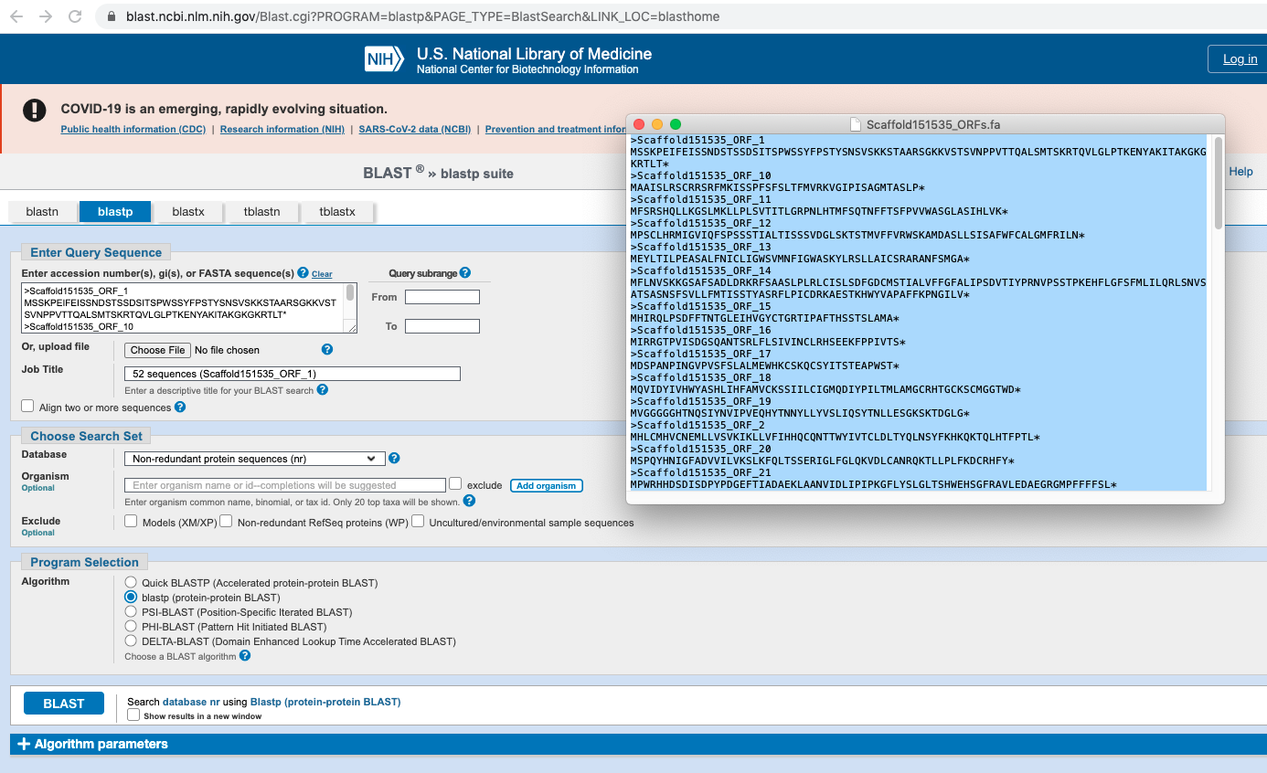
Figure 12.2: Online protein BLAST form.
- Inspect output of protein BLAST analysis and identified ORF(s) along scaffold coding for Aquaporin gene products (see Figure 12.3).
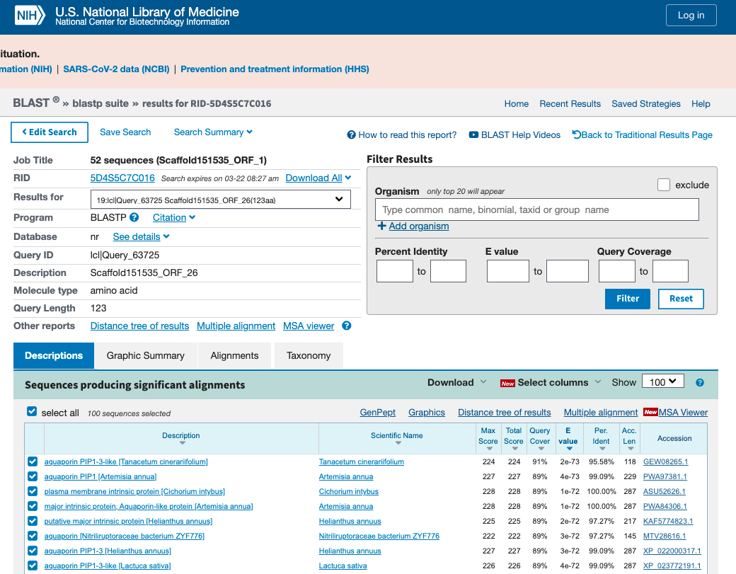
Figure 12.3: Output of the protein BLAST analysis. Use the dropdown button to select each ORF and identify their gene products.
- What ORFs are coding for Aquaporin gene products?
12.2.3 Questions
How many ORFs on
Scaffold151535are coding for AQP exons and which are they?
Based on the BLAST analysis and the ORFs map (Figure 11.1), do you predict that the Aquaporin gene sequence in
Scaffold151535is complete or not? Please motivate your answer
12.3 Extract ORF(s) identified by protein BLAST analysis to reconstruct Aquaporin gene sequence
Students are tasked to develop an R code producing the AA sequence of Aquaporin gene located on identified scaffold and its associated protein sequence.
12.4 A user-defined function to produce a protein sequence
Please find below a user defined function (UDF) that concatenates ORFs into a protein sequence in FASTA format. This function implements defensive programming aiming at providing the users with meaningful error messages to debug their code.
In this UDF, defensive programming has been implemented 2-ways:
- The code checks that the
FASTAfile declared infastaAAexists in the working directory (or in the provided path) and stops and return an error message pertaining to this issue if it doesn’t. - The code checks that all the ORFs declared in
ORFsToCatexists in the FASTA file (= declared infastaAA) and stops and return an error message pertaining to this issue if they are not all present in the file.
Finally, the UDF as a logical argument entitled stopCodon allowing to declare whether stop codons (represented by *) are present in the AA sequences (in your FASTA file). Here it is especially convenient since the concatenated protein sequence should not contain stop codons for our subsequent analyses. See UDF below for more details.
The function is provided below for you to inspect and understand the approach and its implementation. Do not include this code in your script, as it is intended for reference purposes only.
###~~~~
#ORFs2protSeq - A UDF to produce a protein sequence from ORFs
# Arguments:
# - fastaAA: Name of Fasta file containing ORFs AA sequences
# - ORFsToCat: vector with names of ORFs to concatenate (as in FASTA file and including ">" and in the right order)
# - stopCodon: Logical (TRUE/FALSE) variable to state whether stop (*) codons are in the AA sequences
# Output:
# - An object with the concatenated protein sequence in FASTA format
ORFs2protSeq <- function(fastaAA, ORFsToCat, stopCodon){
  #Check if the FASTA file exists
  checkFile <- file.exists(fastaAA)
  if(checkFile == FALSE){
    #Stop the function and print error
    stop(call. = FALSE, paste(fastaAA, "does not exists! Please check that your working directory is set properly.", sep = " "))
  }else{
    #Open FASTA file
    fas <- readLines(fastaAA)
    #Find ORFs in Fasta file
    ToFind <- match(ORFsToCat, fas)
    #Check that all the ORFs were found in the Fasta
    checkORFs <- is.na(ToFind)
    if(length(which(checkORFs == TRUE)) > 0){
      #Stop the function and print error
      stop(call. = FALSE, paste(paste(ORFsToCat[which(checkORFs == TRUE)], collapse = " "), "couldn't be found in", fastaAA, " Please fix the error(s).", sep = " "))
    }else{
      print(paste("Producing protein sequence with", paste(ORFsToCat, collapse = ", "), sep = " "))
      #Cat ORFs into AA sequence
      protSeq <- paste(fas[ToFind+1], collapse = "")
      if(is.logical(stopCodon) == TRUE){
        #Discard stop codons from final sequence
        protSeq <- gsub("[*]", "", protSeq)
      }
    }
    #Produce final protein sequence in FASTA format
    # header
    head <- paste(">Protein_sequence_from_", paste(gsub("[>]", "", ORFsToCat), collapse = "|"), sep= "")
    protSeqOUT <- paste(head, protSeq, sep = "\n")
    print(protSeqOUT)
  }
  return(protSeqOUT)
}
12.4.1 Bioinformatics
In this section, we apply the UDF ORFs2protSeq to Scaffolds_groups.fasta (= fastaAA). First, we will use an example where the ORFsToCat argument contains ORFs that are not found in the FASTA file to demonstrate how defensive programming was implemented in the UDF.
The step-by-step approach is as follows:
Copy the UDF ORFs2protSeq() in your R code and execute it to source the function in the global environment (on the remote computer)
Apply ORFs2protSeq() to a FASTA file containing ORFs
#Name of the FASTA file (make sure the path is correct)
fastaAA <- "Data/Scaffold151535_ORFs.fa"

#Fasta headers of the ORFs you want to concatenate
# Here some ORFs names are faulty
ORFsToCat <- c(">Scaffold151535_ORF_1tt", ">Scaffold151535_ORF_13c", ">Scaffold151535_ORF_2")

#Stop codon
stopCodon <- TRUE

#Apply UDF
ORFs2protSeq(fastaAA, ORFsToCat, stopCodon)
## Error: >Scaffold151535_ORF_1tt >Scaffold151535_ORF_13c couldn't be found in Data/Scaffold151535_ORFs.fa Please fix the error(s).- Apply the UDF again, but this time with matching ORFs (= they are declared in the
FASTAfile)
#Name of the FASTA file
fastaAA <- "Data/Scaffold151535_ORFs.fa"

#Fasta headers of the ORFs you want to concatenate
# Here ORF names are accurate
ORFsToCat <- c(">Scaffold151535_ORF_1", ">Scaffold151535_ORF_13", ">Scaffold151535_ORF_2")

#Stop codon
stopCodon <- TRUE

#Apply UDF
ORFs2protSeq(fastaAA, ORFsToCat, stopCodon)
## [1] "Producing protein sequence with >Scaffold151535_ORF_1, >Scaffold151535_ORF_13, >Scaffold151535_ORF_2"
## [1] ">Protein_sequence_from_Scaffold151535_ORF_1|Scaffold151535_ORF_13|Scaffold151535_ORF_2\nMSSKPEIFEISSNDSTSSDSITSPWSSYFPSTYSNSVSKKSTAARSGKKVSTSVNPPVTTQALSMTSKRTQVLGLPTKENYAKITAKGKGKRTLTMEYLTILPEASALFNICLIGWSVMNFIGWASKYLRSLLAICSRARANFSMGAMHLCMHVCNEMLLVSVKIKLLVFIHHQCQNTTWYIVTCLDLTYQLNSYFKHKQKTQLHTFPTL"## [1] ">Protein_sequence_from_Scaffold151535_ORF_1|Scaffold151535_ORF_13|Scaffold151535_ORF_2\nMSSKPEIFEISSNDSTSSDSITSPWSSYFPSTYSNSVSKKSTAARSGKKVSTSVNPPVTTQALSMTSKRTQVLGLPTKENYAKITAKGKGKRTLTMEYLTILPEASALFNICLIGWSVMNFIGWASKYLRSLLAICSRARANFSMGAMHLCMHVCNEMLLVSVKIKLLVFIHHQCQNTTWYIVTCLDLTYQLNSYFKHKQKTQLHTFPTL"- Modify the code above to save the output of ORFs2protSeq() as a
FASTAfile at a specified path on your remote computer. The input fileScaffold151535_ORFs.fais located in~/DraftGenomeMineR/AA_ORFs. When modifying the code provided above, you may use thewrite.table()function to save the protein sequences in the same directory. For additional guidance, refer to step 2 of Section 11.3.2.
Note: The code provided above is for reference only to help you understand the approach and its implementation. Do not include it directly in your script.
13 Module 4
13.1 Objectives
The objectives of this module are to validate the AQP protein sequences obtained in module 3 (available in ~/DraftGenomeMineR/AA_ORFs) and infer its function. This will be done by conducting the following analyses:
- Predict the number of protein transmembrane helices based on the approach implemented in TMHMM (Krogh et al., 2001). This approach relies on Hidden Markov Models.
- Identify NPA motifs using an
Rscript relying on Biostring (Pagès et al., 2019) and IRanges (Lawrence et al., 2013) packages. - Model 3D AQP protein using an approach implemented in Phyre2 and predict protein (therefore its function). The approach for protein modeling, prediction and analysis is presented in Kelley et al. (2015).
13.1.1 Predictions
To be valid, the AQP protein sequence should have:
- Six transmembrane helices.
- Two hydrophobic loops.
- Two NPA motifs (one per loop).
- Mutations in the NPA motifs (at N or A positions) changes affinity with water and therefore suggests different substrate (i.e., this would be indicative of a change of function).
13.2 Predict the number of protein transmembrane helices (THM) (and outside loops)
To conduct this analysis (based on >Scaffold151535_ORF_26) do the following:
- Go to the TMHMM website: https://services.healthtech.dtu.dk/service.php?TMHMM-2.0
- Paste the
FASTAAA sequence generated in module 3, here corresponding toScaffold151535_ORF_26as shown in Figure 13.1 and submit the analysis.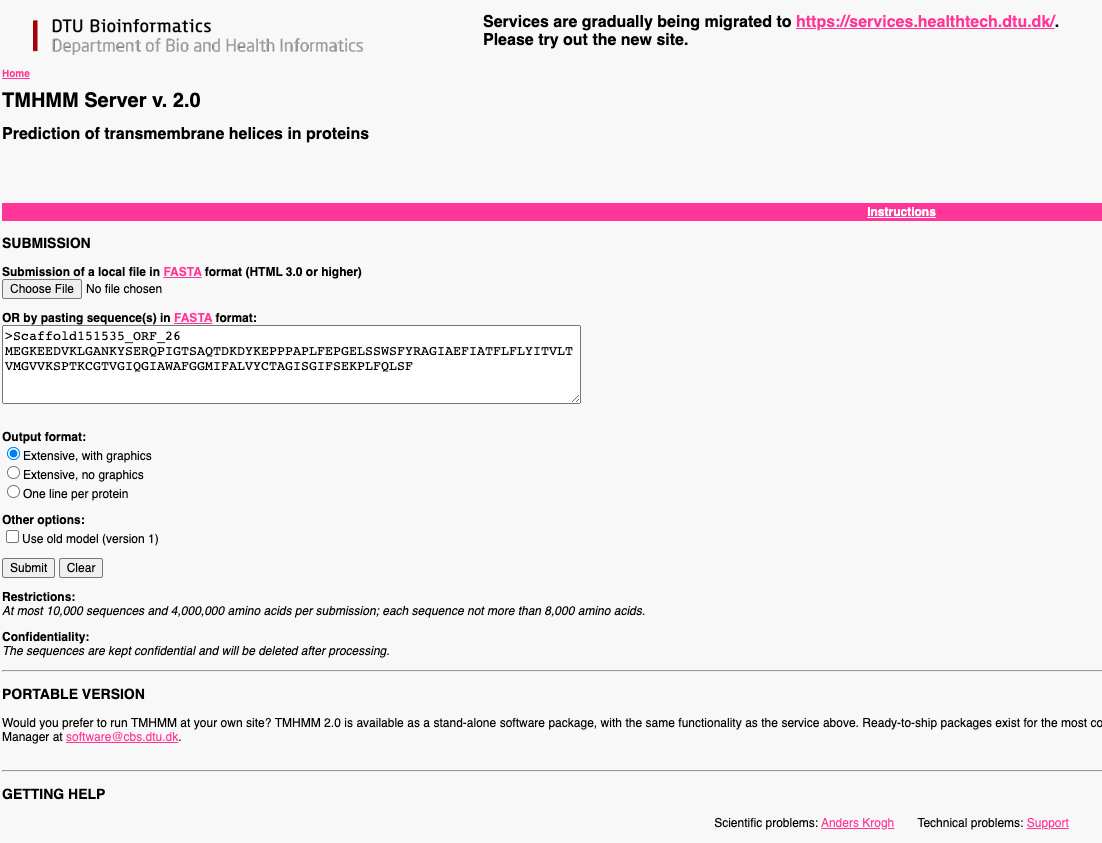
Figure 13.1: Snapshot of TMHMM website showing how to submit job.
- Inspect the output of the TMHMM analysis (see Figure 13.2). For AQP proteins, we are expecting:
- Number of predicted TMHs (= Trans-Membrane Helix): 6.
- Outside loops: 2.
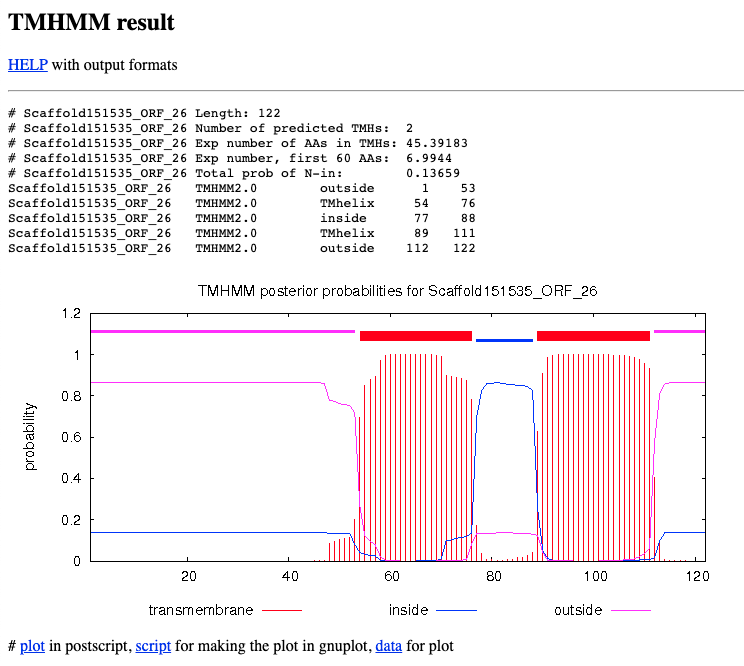
Figure 13.2: Snapshot of TMHMM results.
13.3 Identify the number of NPA motifs and type
In this section, we are identifying the location and type of NPA motif along the AQP protein sequence. The instructors provide a template of an R code (based on Scaffold151535_ORF_26) to conduct this task relying on the Biostring (Pagès et al., 2019) and IRanges (Lawrence et al., 2013) packages. These latter packages should already be installed on your computer, but if they are not then install and load them as follows:
#Install Biostrings and IRanges (deposited on Bioconductor)
BiocManager::install("Biostrings")
BiocManager::install("IRanges")

#Load the packages to check installation
pkgs <- c("Biostrings", "IRanges")
lapply(pkgs, require, character.only = TRUE)
Now that the R packages are installed and loaded we can carry on with our coding:
##
#AA sequence
##
#User copy AA sequence in the object below
# Here, associated to Scaffold151535_ORF_26
AAseq <- "MEGKEEDVKLGANKYSERQPIGTSAQTDKDYKEPPPAPLFEPGELSSWSFYRAGIAEFIATFLFLYITVLTVMGVVKSPTKCGTVGIQGIAWAFGGMIFALVYCTAGISGIFSEKPLFQLSF*"

##
#Create a data.frame to store data on
# - N_NPA: Number of NPA motifs
# - NPA_motif: NPA motif
# - StartNPA: Starting position of NPA motif in AA seq
##
NPAdat <- data.frame("N_NPA" = numeric(length(AAseq)), "NPA_motif" = character(length(AAseq)), "StartNPA" = numeric(length(AAseq)))

#Start by matching to find NP motif and locations along sequence
tmp <- Biostrings::matchPattern(pattern = "NP", Biostrings::AAString(AAseq))
tmp <- as.data.frame(IRanges::ranges(tmp))

if(nrow(tmp) > 0){
  #Print that it found NP motif
  print("NP found")
  #There is an NP motif
  #N NP
  NPAdat$N_NPA <- nrow(tmp)
  #Infer motifs
  NPAdat$NPA_motif <- paste(paste(rep("NP", nrow(tmp)), strsplit(as.vector(AAseq), split='')[[1]][as.numeric(tmp[,2]+1)], sep = ''), collapse = '/')
  #Start motifs
  NPAdat$StartNPA <- paste(tmp[,1], collapse = '/')
  }else{
    #There isn't an NP motif, so we look for a PA motif
  tmp <- Biostrings::matchPattern(pattern = "PA", Biostrings::AAString(AAseq))
  tmp <- as.data.frame(IRanges::ranges(tmp))
      if(nrow(tmp) > 0){
      #Print that it found PA motif
      print("PA found")
      #N NP
      NPAdat$N_NPA <- nrow(tmp)
      #Infer motifs
      NPAdat$NPA_motif <- paste(paste(strsplit(as.vector(AAseq), split='')[[1]][as.numeric(tmp[,1]-1)], rep("PA", nrow(tmp)), sep = ''), collapse = '/')
      #Start motifs
      NPAdat$StartNPA <- paste(tmp[,1]-1, collapse = '/')
      }else{
        next
      }
}
## [1] "PA found"print(paste("The following NPA motifs were found for AA sequence:", AAseq, sep=" "))## [1] "The following NPA motifs were found for AA sequence: MEGKEEDVKLGANKYSERQPIGTSAQTDKDYKEPPPAPLFEPGELSSWSFYRAGIAEFIATFLFLYITVLTVMGVVKSPTKCGTVGIQGIAWAFGGMIFALVYCTAGISGIFSEKPLFQLSF*"print(NPAdat)## N_NPA NPA_motif StartNPA
## 1 1 PPA 35##
#Write data out
##
# If you want to write the data, execute the following command (don't forget to adjust your path)
#write.csv(NPAdat, file='Scaffold151535_ORF_26_NPA_motifs.csv', row.names = F, quote = F)13.3.1 Question
Based on your number of NPA motifs, how many hydrophobic loops does your Aquaporin protein contain? How does this result compare with the output of the TMHMM analysis?
13.4 Model 3D AQP protein
To model 3D structure of AQP protein and predict its function do the following (here based on >Scaffold151535_ORF_26):
- Go to Phyre2 website: http://www.sbg.bio.ic.ac.uk/~phyre2/html/page.cgi?id=index
- Copy only the AA sequence (without the FASTA header) and fill the form as shown in Figure 13.3. Once completed, please submit job by pressing
Phyre Search. The job will take ca. 50 minutes to run.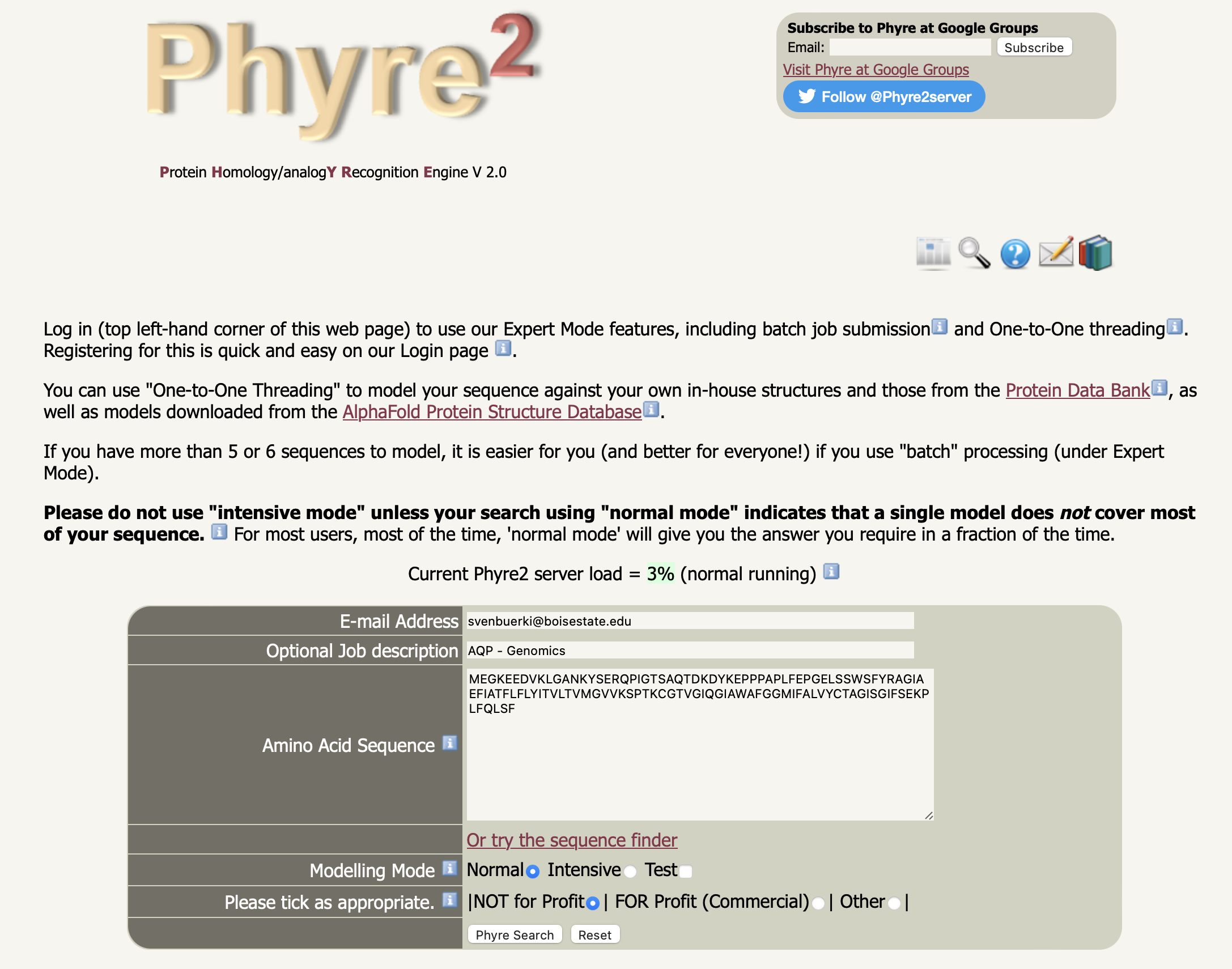
Figure 13.3: Snapshot of Phyre2 website used to model 3D structure of protein and predict its function.
- You will relieve an email when the analysis is completed. A link to the output of the Phyre2 analysis will send you to the report page as shown in Figure 13.4.
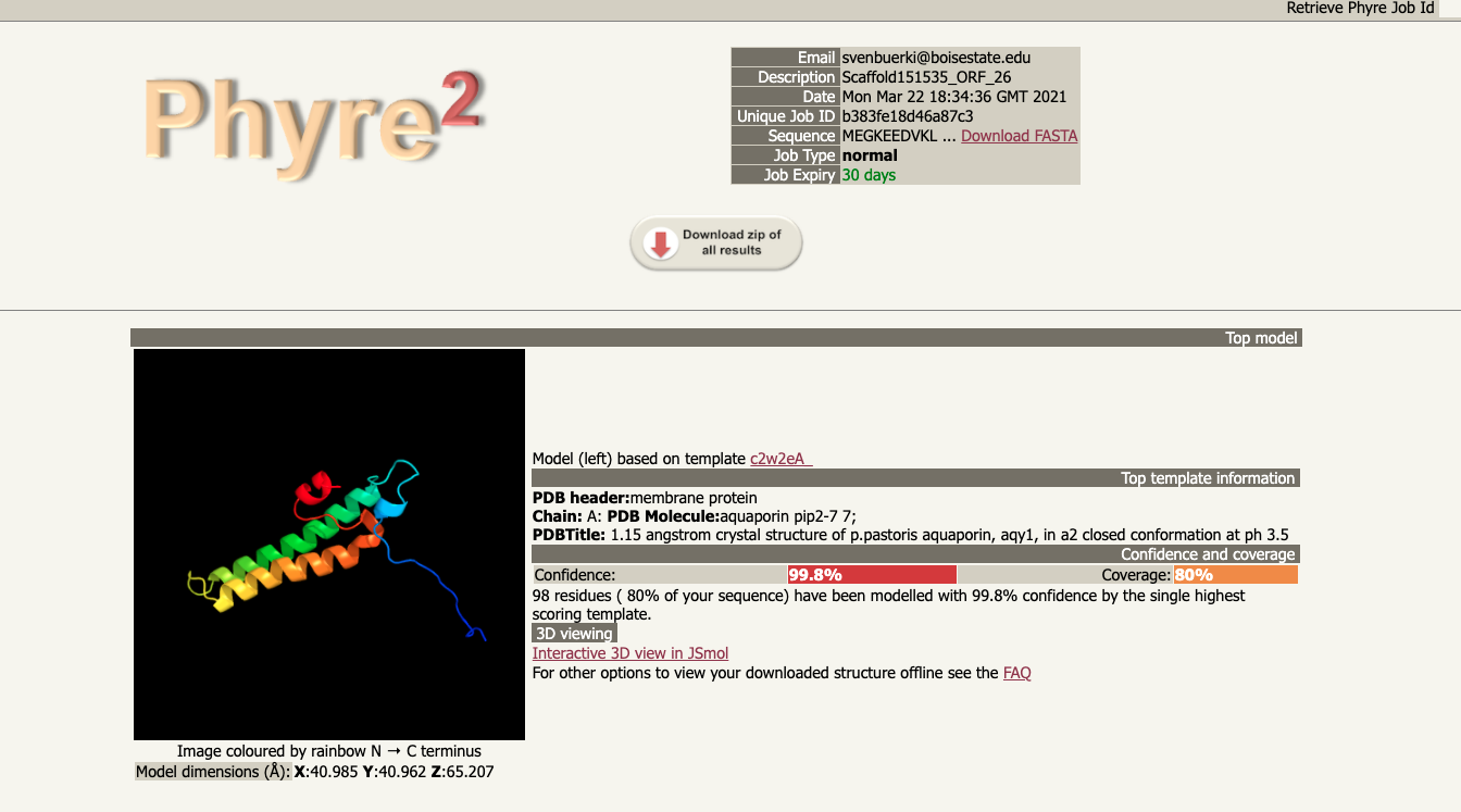
Figure 13.4: Results of Phyre2 analysis.
- Note that although the AQP protein sequence is not complete, the analysis still modeled it correctly and predicted that it belonged to the PIP subfamily (see Figure 13.4).
14 Data Interpretation
Based on the analyses and data gathered in this lab, what are your interpretations and conclusions on the Aquaporin gene/protein located on
Scaffold151535?
Examples of questions that we could ask ourselves to answer the above question are:
- How many Aquaporin exons were recovered and where are they located on the scaffold?
- How many TMHs and loops were inferred?
- How many NPA motifs and types were inferred?
- What is the predicted protein and its function based on the modeling analysis conducted on the AA sequence?
Based on these latter evidence, do you think that the Aquaporin protein sequence is complete? The instructor invites you to consult Melton et al. (2021) for more information allowing answering these questions and come to a conclusion.
15 Your Turn!
Each group is now working as a team to reproduce the analyses presented here on their assigned scaffold.
Good luck!
15.1 Scaffolds assigned to groups
The FASTA file with scaffolds sequences can be downloaded here. The scaffolds assigned to each group are as followed:
- Group 1: Scaffold106379.
- Group 2: Scaffold254734.
- Group 3: Scaffold348135.
16 Group Lab Report Rubric (TOTAL: 150 points)
The instructor provides below information to complete the group report. All the material, data, code and references required to complete this report are provided here and are covered in class. In this context, students will have to focus on formatting their reports following guidelines presented here as well as making sure that their code is working and ready to be shared. Please DON’T FORGET TO PROVIDE REFERENCES FOR SOFTWARE/PACKAGES cited in the Material & Methods section.
16.1 Apply the IMRAD format and supply data and code
Your group reports will be structured and organized following the IMMRAD format: Introduction, Material & Methods, Results, and Discussion. This format is widely used to report experimental research in many scientific disciplines. In addition, you will be complementing your reports with an Abstract. Finally, since this research relies heavily on bioinformatics, students will complete their reports by supplying their data and commented code/scripts. Please see Mini-Report 3 for more details.
Please see evaluation rubrics for more information on grading.
16.2 Report Deadline
Please see here for details on the deadline for this mandatory group assignment.
17 Group Lab Oral Presentation (TOTAL: 50 points)
Students will use their lab reports to prepare a 15-minute group presentation (+ 5 minutes for questions), scheduled for April 29th, 2026 (during class time).
This assignment requires groups to clearly communicate their research following the scientific process (IMRAD structure). Additional details on presentation format, slide organization, and expectations are provided in the sections below and in the evaluation rubrics. The evaluation form used to grade this assignment can be downloaded here.
Participation: All group members are expected to actively contribute to the presentation and participate in answering questions.
Submission: Presentations must be submitted in advance to the shared Google Drive folder.
Please refer to the evaluation rubrics for full grading criteria and performance expectations.
18 Evaluation Rubrics
This section provides the evaluation rubrics for both your group lab reports and oral presentations. Please review them carefully before submitting your final group report and preparing your oral presentation.
18.1 Group Lab Report (Total: 150 points)
Your group lab report will be evaluated based on your ability to communicate a genome mining investigation clearly, accurately, and professionally using the IMRAD format (Introduction, Materials & Methods, Results, Discussion), and by providing reproducible data and code.
Each section is evaluated independently as outlined below.
18.1.1 Abstract (10 points)
| Criteria | Description | Points |
|---|---|---|
| Summary of study | Clearly summarizes the research question, methods, key results, and conclusions | 10 |
18.1.2 Introduction (25 points)
| Criteria | Description | Points |
|---|---|---|
| Scientific context and background | Clearly explains genome mining, gene annotation, and validation in the context of the study organism and target gene family | 10 |
| Research question and objectives | Clearly states the scientific question, objectives, and biological relevance of the investigation | 10 |
| Clarity and organization | Logical structure, clear writing, and appropriate use of scientific terminology | 5 |
18.1.3 Materials & Methods (35 points)
| Criteria | Description | Points |
|---|---|---|
| Description of analytical workflow | Clearly and accurately describes genome mining, scaffold extraction, ORF prediction, annotation, and validation procedures | 15 |
| Reproducibility and transparency | Methods are described with sufficient detail to allow replication, including software, versions, parameters, and databases used | 10 |
| Code quality and documentation | Code/scripts are complete, functional, well-organized, and appropriately commented | 5 |
| Software and database citations | Proper citation of software, packages, and databases used | 5 |
18.1.4 Results (35 points)
| Criteria | Description | Points |
|---|---|---|
| Presentation of genome mining results | Clearly presents scaffold identification, ORF prediction, gene annotation, and validation results | 15 |
| Figures and tables | Figures and tables are clear, correctly labeled, and effectively support the findings | 10 |
| Accuracy and completeness | Results are accurate, complete, and presented without interpretation | 10 |
18.1.5 Discussion (35 points)
| Criteria | Description | Points |
|---|---|---|
| Interpretation of findings | Clearly explains the biological meaning of the identified and validated genes | 15 |
| Integration with scientific context | Connects findings to genome biology, gene function, and the original research question | 10 |
| Critical thinking | Discusses limitations, uncertainties, and potential future directions | 5 |
| Clarity and organization | Logical flow and clear scientific writing | 5 |
18.1.6 Reproducibility: Data and Code Submission (10 points)
| Criteria | Description | Points |
|---|---|---|
| Data submission | Required data files are complete, organized, and accessible | 5 |
| Code submission | Scripts are functional, organized, and allow reproduction of analyses | 5 |
18.1.7 Formatting and Submission Penalties
The following penalties may be applied:
| Issue | Penalty |
|---|---|
| Failure to follow formatting guidelines | Up to −15 points |
| Missing or incomplete code/data | Up to −15 points |
| Missing references or improper citation | Up to −10 points |
| Late submission | see Late Work Policy |
18.2 Group Lab Oral Presentation Rubric (Total: 50 points)
Presentation Length: 15 minutes, plus 5 minutes for questions
Slide Guidelines: Presentations should follow the IMRAD structure (Introduction, Methods and Materials, Results, and Discussion) and be limited to a maximum of 6 slides total (excluding animations and transitions). As a guideline, allocate approximately:
- Introduction: up to 2 slides
- Methods and Materials: up to 2 slides
- Results and Discussion: up to 2 slides
Expectations: All group members must actively participate in the presentation and be prepared to respond to questions. Presentations must be submitted in advance to the shared Google Drive folder or sent to the instructor.
The presentation will be evaluated based on how clearly and professionally the group communicates its research using the scientific process (IMRAD structure), adheres to the slide guidelines, and engages the audience.
The evaluation form used to grade this assignment can be downloaded here.
18.2.1 Introduction & Background (10 points)
| Criteria | Description | Points |
|---|---|---|
| Scientific context | Explains the relevant genome biology, gene annotation, and study organism clearly, providing necessary background | 5 |
| Research question & objectives | Clearly states the research question, objectives, and biological relevance | 3 |
| Clarity and engagement | Information is logically organized, concise, and engages the audience | 2 |
18.2.2 Materials & Methods (10 points)
| Criteria | Description | Points |
|---|---|---|
| Explanation of workflow | Clearly describes genome mining, ORF prediction, annotation, and validation steps appropriate for oral communication | 5 |
| Reproducibility and transparency | Describes tools, software, and databases used with enough detail for comprehension | 3 |
| Clarity & conciseness | Methods are presented in an understandable, well-structured way for the audience | 2 |
18.2.3 Results (12 points)
| Criteria | Description | Points |
|---|---|---|
| Presentation of findings | Results are clearly explained, including scaffold identification, gene annotation, and validation | 5 |
| Visual aids | Figures, tables, and slides are clear, correctly labeled, and enhance audience understanding | 4 |
| Accuracy & completeness | Results are accurate and complete, presented without misinterpretation | 3 |
18.2.4 Discussion & Interpretation (10 points)
| Criteria | Description | Points |
|---|---|---|
| Interpretation of findings | Clearly explains biological significance and connects to research question | 5 |
| Integration with context | Connects results to genome biology, gene function, or broader implications | 3 |
| Critical thinking | Discusses limitations, uncertainties, and potential next steps | 2 |
18.2.5 Communication & Engagement (8 points)
| Criteria | Description | Points |
|---|---|---|
| Participation | All group members contribute and respond to questions | 3 |
| Clarity & delivery | Speech is clear, confident, and well-paced; avoids excessive reading from slides | 3 |
| Audience engagement | Effectively engages listeners, maintains attention, and handles questions professionally | 2 |
18.2.6 Formatting and Submission Penalties (Optional)
| Issue | Penalty |
|---|---|
| Exceeding 10-minute presentation time | Up to −3 points |
| Failing to present | see Late Work Policy |
19 Acknowledgements
The instructor would like to thank Dr Anthony Melton (University of Montevallo, Montevallo, AL) for his incredible support with the analyses presented in this group activity.