Biomass production
1 Biomass requirements for genome project
We aim at applying the newly developed in vitro tissue culture technique (Barron et al., 2020) to the G2_b24_1 individual line (from UTT2, drought-sensitive genotype; see Figure 1.1) to produce the ca. 120 gr of leaf biomass necessary for genome sequencing, phasing and annotation. As mentioned in our introduction, we also need to make sure that we are maintaining the individual line beyond biomass production to support genome to phenome research (based on GxE experiments).
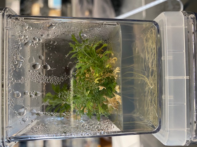
Figure 1.1: Example of a 15-week old plantlet grown in vitro in Magenta vessel.
1.1 Adapting approach to biomass production
Our propagation method (see here for more details) to maintain individual line in vitro works very well, but after 8-10 weeks of growth a plantlet only generates ca. 0.15 gr of biomass for genome sequencing. This is only when allocating 1 plantlet per Magenta vessel. Indeed, sagebrush are competing using chemical compounds and putting several individuals per Magenta vessel decreases growth and increases mortality. Overall, if we were to apply to approach to generate the necessary 120 gr for the sagebrush genome project, we would need 800 plantlets. This large number of plantlet is logistically challenging and could prove difficult to handle for our small to middle size lab. This is even more challenging because although our methodology has a high (>90%) rooting response, the survival rate during the growth step is highly variable between individual lines. For instance, the top performer as identified by Barron et al. (2020), G2_b27_1, has only a 45% survival rate in the second round of propagation, whereas G2_b24_1 has a 80% survival rate at the same stage. This evidence means that far more plantlets would have to be cultivated to reach the 800 plantlets mark (corresponding to 120 gr.). This latter estimate is without accounting for a cushion to maintain the individual line for genome to phenome research. In this context, we have favored i) selecting an individual with a high survival rate and ii) growing plantlets for a longer period to obtain more biomass. To differentiate this stage of the propagation to our regular steps, we will be referring to the allocation of plantlets to biomass production as biobanking (see below for more details).
1.1.1 Using 15-week old G2_b24_1 plantlets to produce biomass
After 15 weeks of in vitro tissue culture, a plantlet produces ca. 0.8 gr. of leaf biomass that can be used for sequencing (Figure 1.2). Thus, a minimum of 150 plantlets have to be produced to sequence the genome (see Table ??). This number is much more manageable and means that all the plantlets can be grown in individual Magenta vessels under optimum growth conditions in our Percival culture chamber. When ready, the biomass will be flash frozen (using liquid nitrogen) and stored at -80C before being shipped to the sequencing facility. However, the estimation of biomass provided here does not account for a DNA extraction trial required to optimize protocol (we need at least 15µg of HMW DNA for PacBio sequencing). We will have to discuss this with the project manager at Dovetail Genomics.
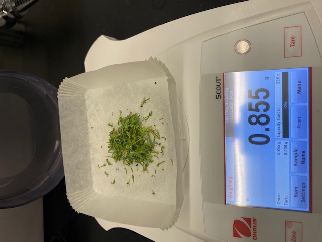
Figure 1.2: A 15-week old plantlet grown in vitro in Magenta vessel generates 0.8 gr of leaf biomass for sequencing.
2 Planning biomass production for sequencing
To be able to plan the biomass production for genome sequencing, while also maintaining the individual line, we have developed an R function called propagationPred. This function incorporates 4 steps (Growth, Cutting, Rooting and Biobanking) as well as the rooting and survival rates. In addition, the use can define duration for the Growth, Rooting and Biobanking steps, which allows establishing a schedule. Finally, this function also incorporates details on times necessary for preparing media and number of plates and Magenta vessels required to complete propagation protocols. The function is presented below.
2.1 Presenting R propagationPred function
propagationPred depends on the following set of arguments provided by the user:
n: number of plantlets to seed the experiment.ns: number of shoot tips cut per plantlet (after the growth period).r: vector of rooting rates (0 to 1) at each rooting phase.s: vector of survival rates (0 to 1) at each growth phase.g: number of generations (for in vitro propagation).biobank: vector with proportion (0 to 1) of plantlets biobanked per generation (at end of growth) (e.g: c(0,0,0.4,0)). This argument is important since it is equal to the number of plantlets set aside for biomass production.date_user: starting date of the experiment (mdy from ludridate or any date format).growth_time_g: vector with number of days/weeks allocated for growth perg(how long will it take for your plantlets to producens).biobanking_time: one value (either weeks() or days()) compatible with lubridate describing the duration of biobanking to generated the biomass (here 15 weeks corresponding to 0.8 gr).rooting_time_g: vector with number of days/weeks for rooting perg. The rooting time is a key factor, you want to allocate enough time for roots to develop and growth.biomass_plantlet: numerical value of biomass of a single plantlet (here 0.8 gr).
The function outputs a data.frame with the following columns:
Generation: Generation ID.Type: Type of in vitro activity (Growth,Cutting,Rooting,Biobanking).Date_startandDate_end: Start and end date associated toType.N_plant_startandN_plant_end: Number of plantelts at stat and end dates.N_vessels: Number of plates (forRooting) or Magenta (forGrowth) vessels. 1 plate = 9 shoot tips, whereas rooted shoot tips are on individual Magenta vessels.
Volume_media_litre: Amount ofRooting(0.05 liter per plate) orGrowth(0.1 liter per Magenta vessel) media to be prepared.
N_AutoclaveandTime_Autoclave (hrs): Number of autoclaves used to prepareRooting(1 liter per autoclave) orGrowth(60 Magenta vessels per autoclave) media and associated times (120 minutes forRootingmedia vs. 90 minutes forGrowthmedia).Media_prep_time (hrs)andTime_Cutting (hrs): Lab our time to prepareRooting(90 minutes for 1 liter) orGrowth(1 hr for 60 boxes) media and conduct cutting (5 plantlets per hour).
Total_Biomass (gr): This is estimated based on fraction of plantlets allocated to biobanking (based onbiomass_plantlet).
The output can directly be used to plan in vitro propagation, but can also be easily used as input to produce a plot showing the different steps through time (see below).
3 Scheduling propagation of G2_b24_1
As mentioned above, we have selected the G2_b24_1 individual line as candidate for the Sagebrush Genome Project. In this section, we are using propagationPred to:
- Provide timetable of biomass production, especially to identify when the biomass will be ready to be delivered to Dovetail Genomics for sequencing.
- Logistically organize the biomass production.
3.1 Settings applied for analyses
The propagationPred function has been applied with the following parameters (see section 3.4 for R code):
n: 6 plantlets at generation 1.ns: 9.5 (on average) shoot tips per plantlets after 10 weeks of growth.r: 0.93 rooting rate (same at each generation).s: 0.8 survival rate (same at each generation).g: 4 generations of propagation.biobank: c(0,0,0.9,0). Meaning that 90% of plantlets will be biobanked at generation 3. Based on preliminary analyses, this should provide sufficient number of plantlets for biomass production.date_user: 2020-09-04 is the beginning of growth period at generation 1.growth_time_g: c(weeks(10),weeks(8),weeks(8),weeks(8)).biobanking_time: weeks(15). This corresponds to the duration required for a plantlet to produce 0.8 gr of leaf biomass.rooting_time_g: c(weeks(4),weeks(3),weeks(3),weeks(3)).biomass_plantlet: 0.8 (in gr).
3.2 Timetable of biomass production
A detailed timetable for each steps of the propagation procedure of the G2_b24_1 individual line is available below.
3.2.1 Key highlights
- On 2021-02-26, 333 rooted plantlets transferred into individual Magenta vessels will be biobanked in a dedicated Percival. Based on our prediction, 266 plantlets will survived and produce 212.8 gr. of biomass by 2021-06-11.
- The biomass production should largely exceed the needs of the project, which might suggest that we could deliver the biomass sooner. However, this remains a prediction, which will have to be confirmed.
- To better visualize the timetable, a plot was produced and it highlights the key dates and facts (see Figure 3.1).
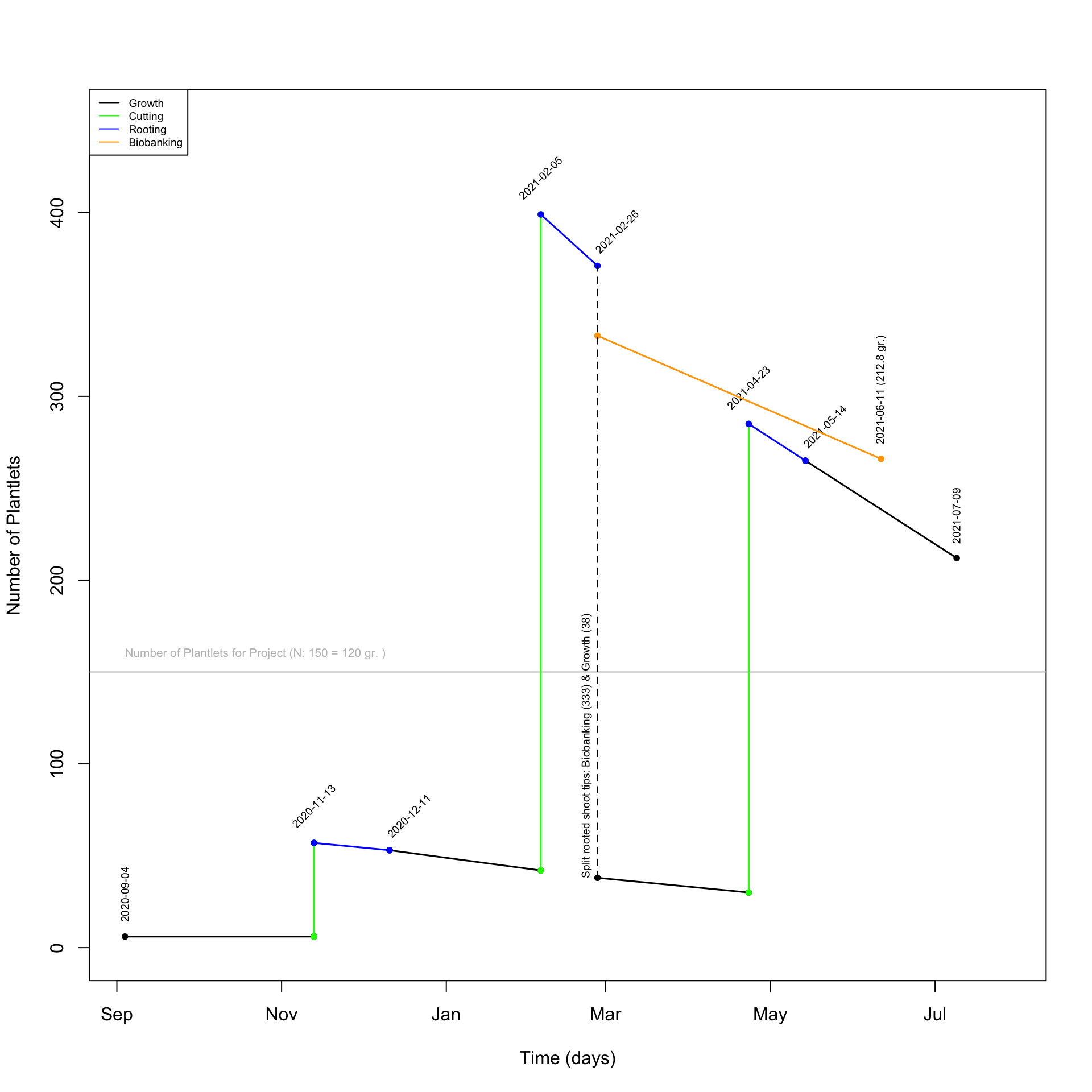
Figure 3.1: Plot showing the time frame to conduct the in vitro propagation of G2_b24_1 to produce the biomass for the Sagebrush Genome Project and maintain the individual line.
3.3 Logistical organization
To prepare with each step of the propagation, we are providing key knowledge in the table below:
3.3.1 Key highlights
- The Cutting on 2021-02-05 will require NA hours of labor. We will have to make sure to coordinate and take 2-3 days to complete this step.
- A total of 399 Magenta vessels will be needed by 2021-02-05.
3.4 R code
#Source user-made function
source("Functions/Propagation.R")

#Apply propagationPred to top performer (G2_b24_1 from UTT2)
OUTdat <- propagationPred(n=6, ns=9.5, r=rep(0.93,4), s=rep(0.8,4), g=4, biobank=c(0,0,0.9,0), date_user=mdy("11/13/2020")-weeks(10), growth_time_g=c(weeks(10),weeks(8),weeks(8),weeks(8)), biobanking_time = weeks(15), rooting_time_g=c(weeks(4),weeks(3),weeks(3),weeks(3)), biomass_plantlet = 0.8)

#Subset OUTdat to only contain rows of interests
OUTdat <- OUTdat[1:11,]

#Plot table
DT::datatable(OUTdat, extensions = 'Buttons', options = list(dom = 'Blfrtip', buttons = c('copy', 'csv', 'excel', 'pdf', 'print')))

###~~~
#Plot data
###~~~
#pdf("Schedule_sagebrush_propagation_G2_b24_1.pdf")
#Populate plot
Type <- levels(OUTdat$Type)[c(3,2,4,1)]
colSeg <- c("black","green","blue","orange")

#Create empty plot
plot(x=c(as.Date(OUTdat$Date_start)), y= c(as.numeric(as.vector(OUTdat$N_plant_start))),
     xlim= c(min(as.Date(OUTdat$Date_start)), max(as.Date(OUTdat$Date_end))+20),
     ylim=c(0, max(as.numeric(as.vector(OUTdat$N_plant_start)))+50), type='n', xlab="Time (days)", ylab = "Number of Plantlets")

biomassTot <- 120
biomass_plantlet <- 0.8
#Add objective of N plantlets
abline(h=biomassTot/biomass_plantlet, col='grey')
text(x=as.Date(OUTdat$Date_start[1]), y=biomassTot/biomass_plantlet+10, labels=paste("Number of Plantlets for Project (N: ", biomassTot/biomass_plantlet, " = ", biomassTot, " gr. )", sep=""), adj=0, col="grey", cex=.65)

#Add segments
for(i in 1:length(Type)){
  tmp <- OUTdat[which(OUTdat$Type == Type[i]),]
  segments(x0=as.Date(tmp$Date_start), x1=as.Date(tmp$Date_end), y0=as.numeric(as.vector(tmp$N_plant_start)), y1=as.numeric(as.vector(tmp$N_plant_end)), col=colSeg[i], lwd=1.5)
  #Add points to better see beginning and end of phases
  points(x=as.Date(tmp$Date_start), y=as.numeric(as.vector(tmp$N_plant_start)), col=colSeg[i], pch=16, cex=.8)
  points(x=as.Date(tmp$Date_end), y=as.numeric(as.vector(tmp$N_plant_end)), col=colSeg[i], pch=16, cex=.8)

  if(Type[i] == "Cutting"){
    text(x=as.Date(tmp$Date_start), y=as.numeric(as.vector(tmp$N_plant_end))+20, labels = as.Date(tmp$Date_start), srt=45, adj=0.5, cex=.6)
  }
  if(Type[i] == "Rooting"){
    text(x=as.Date(tmp$Date_end), y=as.numeric(as.vector(tmp$N_plant_end))+8, labels = as.Date(tmp$Date_end), srt=45, adj=0, cex=.6)
  }
  if(Type[i] == "Growth"){
    #Start of experiment
    startExp <- which(tmp$Date_start == as.character(min(as.Date(tmp$Date_start))))
    text(x=as.Date(tmp$Date_start)[startExp], y=as.numeric(as.vector(tmp$N_plant_start))[startExp]+8, labels = as.Date(tmp$Date_start)[startExp], srt=90, adj=0, cex=.6)

    #End of experiment
    endExp <- which(tmp$Date_end == as.character(max(as.Date(tmp$Date_end))))
    text(x=as.Date(tmp$Date_end)[endExp], y=as.numeric(as.vector(tmp$N_plant_end))[endExp]+8, labels = as.Date(tmp$Date_end)[endExp], srt=90, adj=0, cex=.6)
  }
  if(Type[i] == "Biobanking"){
    #Add segment(s) showing when rooted shoot tips are split between growth and biobanking
    ystart <- as.numeric(as.vector(OUTdat$N_plant_start[which(OUTdat$Date_start == tmp$Date_start & OUTdat$Type == "Growth")]))
    yend <- as.numeric(as.vector(OUTdat$N_plant_end[which(OUTdat$Date_end == as.character(tmp$Date_start) & OUTdat$Type == "Rooting")]))
    segments(x0=as.Date(tmp$Date_start), x1=as.Date(tmp$Date_start), y0=ystart, y1=yend, lty=2)
    text(x=as.Date(tmp$Date_start)-4, y=ystart, paste("Split rooted shoot tips:", paste(as.character(tmp$Type), " (", tmp$N_plant_start, ")", " & Growth (", ystart, ")", sep="")), adj=0, srt=90, cex=.6)

    #End of experiment
    endExp <- which(tmp$Date_end == as.character(max(as.Date(tmp$Date_end))))
    text(x=as.Date(tmp$Date_end)[endExp], y=as.numeric(as.vector(tmp$N_plant_end))[endExp]+8, labels = paste(as.Date(tmp$Date_end)[endExp], " (", as.character(tmp$`Total_Biomass (gr)`), " gr.)", sep=''), srt=90, adj=0, cex=.6)
  }

}

#Add legend
legend("topleft", legend = Type, lty=1, col=colSeg, cex=.6)
#dev.off()
4 References
5 Appendix 1
Citations of all R packages used to generate this report.
[1] J. Allaire, Y. Xie, J. McPherson, et al. rmarkdown: Dynamic Documents for R. R package version 2.6. 2020. <URL: https://github.com/rstudio/rmarkdown>.
[2] C. Boettiger. knitcitations: Citations for Knitr Markdown Files. R package version 1.0.10. 2019. <URL: https://github.com/cboettig/knitcitations>.
[3] J. Bryan. googlesheets4: Access Google Sheets using the Sheets API V4. R package version 0.2.0. 2020. <URL: https://github.com/tidyverse/googlesheets4>.
[4] J. Cheng, B. Karambelkar, and Y. Xie. leaflet: Create Interactive Web Maps with the JavaScript Leaflet Library. R package version 2.0.3. 2019. <URL: http://rstudio.github.io/leaflet/>.
[5] D. Ebbert. chisq.posthoc.test: A Post Hoc Analysis for Pearson’s Chi-Squared Test for Count Data. R package version 0.1.2. 2019. <URL: http://chisq-posthoc-test.ebbert.nrw/>.
[6] G. Grolemund and H. Wickham. “Dates and Times Made Easy with lubridate.” In: Journal of Statistical Software 40.3 (2011), pp. 1-25. <URL: https://www.jstatsoft.org/v40/i03/>.
[7] T. Hothorn, A. Zeileis, R. W. Farebrother, et al. lmtest: Testing Linear Regression Models. R package version 0.9-38. 2020. <URL: https://CRAN.R-project.org/package=lmtest>.
[8] S. Jackman, A. Tahk, A. Zeileis, et al. pscl: Political Science Computational Laboratory. R package version 1.5.5. 2020. <URL: http://github.com/atahk/pscl>.
[9] A. Kassambara. ggpubr: ggplot2 Based Publication Ready Plots. R package version 0.4.0. 2020. <URL: https://rpkgs.datanovia.com/ggpubr/>.
[10] M. C. Koohafkan. kfigr: Integrated Code Chunk Anchoring and Referencing for R Markdown Documents. R package version 1.2. 2015. <URL: https://github.com/mkoohafkan/kfigr>.
[11] R. Lenth. emmeans: Estimated Marginal Means, aka Least-Squares Means. R package version 1.5.2-1. 2020. <URL: https://github.com/rvlenth/emmeans>.
[12] R. Lenth. lsmeans: Least-Squares Means. R package version 2.30-0. 2018. <URL: https://CRAN.R-project.org/package=lsmeans>.
[13] R. V. Lenth. “Least-Squares Means: The R Package lsmeans.” In: Journal of Statistical Software 69.1 (2016), pp. 1-33. DOI: 10.18637/jss.v069.i01.
[14] E. Neuwirth. RColorBrewer: ColorBrewer Palettes. R package version 1.1-2. 2014. <URL: https://CRAN.R-project.org/package=RColorBrewer>.
[15] E. Paradis, S. Blomberg, B. Bolker, et al. ape: Analyses of Phylogenetics and Evolution. R package version 5.4-1. 2020. <URL: http://ape-package.ird.fr/>.
[16] E. Paradis and K. Schliep. “ape 5.0: an environment for modern phylogenetics and evolutionary analyses in R.” In: Bioinformatics 35 (2019), pp. 526-528.
[17] R Core Team. R: A Language and Environment for Statistical Computing. R Foundation for Statistical Computing. Vienna, Austria, 2019. <URL: https://www.R-project.org/>.
[18] K. Ren and K. Russell. formattable: Create Formattable Data Structures. R package version 0.2.0.1. 2016. <URL: https://CRAN.R-project.org/package=formattable>.
[19] B. Ripley. MASS: Support Functions and Datasets for Venables and Ripley’s MASS. R package version 7.3-53. 2020. <URL: http://www.stats.ox.ac.uk/pub/MASS4/>.
[20] M. R. Smith. TreeTools: Create, Modify and Analyse Phylogenetic Trees. R package version 1.4.0. 2020. <URL: https://CRAN.R-project.org/package=TreeTools>.
[21] V. Spinu, G. Grolemund, and H. Wickham. lubridate: Make Dealing with Dates a Little Easier. R package version 1.7.9.2. 2020. <URL: https://CRAN.R-project.org/package=lubridate>.
[22] W. N. Venables and B. D. Ripley. Modern Applied Statistics with S. Fourth. ISBN 0-387-95457-0. New York: Springer, 2002. <URL: http://www.stats.ox.ac.uk/pub/MASS4/>.
[23] G. R. Warnes, B. Bolker, L. Bonebakker, et al. gplots: Various R Programming Tools for Plotting Data. R package version 3.1.0. 2020. <URL: https://github.com/talgalili/gplots>.
[24] H. Wickham. forcats: Tools for Working with Categorical Variables (Factors). R package version 0.5.0. 2020. <URL: https://CRAN.R-project.org/package=forcats>.
[25] H. Wickham. ggplot2: Elegant Graphics for Data Analysis. Springer-Verlag New York, 2016. ISBN: 978-3-319-24277-4. <URL: https://ggplot2.tidyverse.org>.
[26] H. Wickham. stringr: Simple, Consistent Wrappers for Common String Operations. R package version 1.4.0. 2019. <URL: https://CRAN.R-project.org/package=stringr>.
[27] H. Wickham and J. Bryan. usethis: Automate Package and Project Setup. R package version 2.0.0. 2020. <URL: https://CRAN.R-project.org/package=usethis>.
[28] H. Wickham, W. Chang, L. Henry, et al. ggplot2: Create Elegant Data Visualisations Using the Grammar of Graphics. R package version 3.3.3. 2020. <URL: https://CRAN.R-project.org/package=ggplot2>.
[29] H. Wickham, R. François, L. Henry, et al. dplyr: A Grammar of Data Manipulation. R package version 1.0.2. 2020. <URL: https://CRAN.R-project.org/package=dplyr>.
[30] H. Wickham, J. Hester, and W. Chang. devtools: Tools to Make Developing R Packages Easier. R package version 2.3.2. 2020. <URL: https://CRAN.R-project.org/package=devtools>.
[31] H. Wickham and D. Seidel. scales: Scale Functions for Visualization. R package version 1.1.1. 2020. <URL: https://CRAN.R-project.org/package=scales>.
[32] C. O. Wilke. ggridges: Ridgeline Plots in ggplot2. R package version 0.5.2. 2020. <URL: https://wilkelab.org/ggridges>.
[33] Y. Xie. bookdown: Authoring Books and Technical Documents with R Markdown. ISBN 978-1138700109. Boca Raton, Florida: Chapman and Hall/CRC, 2016. <URL: https://github.com/rstudio/bookdown>.
[34] Y. Xie. bookdown: Authoring Books and Technical Documents with R Markdown. R package version 0.21. 2020. <URL: https://github.com/rstudio/bookdown>.
[35] Y. Xie. Dynamic Documents with R and knitr. 2nd. ISBN 978-1498716963. Boca Raton, Florida: Chapman and Hall/CRC, 2015. <URL: https://yihui.org/knitr/>.
[36] Y. Xie. formatR: Format R Code Automatically. R package version 1.7. 2019. <URL: https://github.com/yihui/formatR>.
[37] Y. Xie. “knitr: A Comprehensive Tool for Reproducible Research in R.” In: Implementing Reproducible Computational Research. Ed. by V. Stodden, F. Leisch and R. D. Peng. ISBN 978-1466561595. Chapman and Hall/CRC, 2014. <URL: http://www.crcpress.com/product/isbn/9781466561595>.
[38] Y. Xie. knitr: A General-Purpose Package for Dynamic Report Generation in R. R package version 1.30. 2020. <URL: https://yihui.org/knitr/>.
[39] Y. Xie, J. Allaire, and G. Grolemund. R Markdown: The Definitive Guide. ISBN 9781138359338. Boca Raton, Florida: Chapman and Hall/CRC, 2018. <URL: https://bookdown.org/yihui/rmarkdown>.
[40] Y. Xie, J. Cheng, and X. Tan. DT: A Wrapper of the JavaScript Library DataTables. R package version 0.16. 2020. <URL: https://github.com/rstudio/DT>.
[41] Y. Xie, C. Dervieux, and E. Riederer. R Markdown Cookbook. ISBN 9780367563837. Boca Raton, Florida: Chapman and Hall/CRC, 2020. <URL: https://bookdown.org/yihui/rmarkdown-cookbook>.
[42] G. Yu and T. T. Lam. ggtree: an R package for visualization of tree and annotation data. R package version 2.0.4. 2020. <URL: https://yulab-smu.github.io/treedata-book/>.
[43] G. Yu, T. T. Lam, H. Zhu, et al. “Two methods for mapping and visualizing associated data on phylogeny using ggtree.” In: Molecular Biology and Evolution 35 (2 2018), pp. 3041-3043. DOI: 10.1093/molbev/msy194. <URL: https://doi.org/10.1093/molbev/msy194>.
[44] G. Yu, D. Smith, H. Zhu, et al. “ggtree: an R package for visualization and annotation of phylogenetic trees with their covariates and other associated data.” In: Methods in Ecology and Evolution 8 (1 2017), pp. 28-36. DOI: 10.1111/2041-210X.12628. <URL: http://onlinelibrary.wiley.com/doi/10.1111/2041-210X.12628/abstract>.
[45] A. Zeileis and G. Grothendieck. “zoo: S3 Infrastructure for Regular and Irregular Time Series.” In: Journal of Statistical Software 14.6 (2005), pp. 1-27. DOI: 10.18637/jss.v014.i06.
[46] A. Zeileis, G. Grothendieck, and J. A. Ryan. zoo: S3 Infrastructure for Regular and Irregular Time Series (Z’s Ordered Observations). R package version 1.8-8. 2020. <URL: http://zoo.R-Forge.R-project.org/>.
[47] A. Zeileis and T. Hothorn. “Diagnostic Checking in Regression Relationships.” In: R News 2.3 (2002), pp. 7-10. <URL: https://CRAN.R-project.org/doc/Rnews/>.
[48] A. Zeileis, C. Kleiber, and S. Jackman. “Regression Models for Count Data in R.” In: Journal of Statistical Software 27.8 (2008). <URL: http://www.jstatsoft.org/v27/i08/>.
[49] H. Zhu. kableExtra: Construct Complex Table with kable and Pipe Syntax. R package version 1.2.1. 2020. <URL: https://CRAN.R-project.org/package=kableExtra>.
6 Appendix 2
Version information about R, the operating system (OS) and attached or R loaded packages. This appendix was generated using sessionInfo().
## R version 3.6.1 (2019-07-05)
## Platform: x86_64-apple-darwin15.6.0 (64-bit)
## Running under: macOS Mojave 10.14.6
##
## Matrix products: default
## BLAS:   /Library/Frameworks/R.framework/Versions/3.6/Resources/lib/libRblas.0.dylib
## LAPACK: /Library/Frameworks/R.framework/Versions/3.6/Resources/lib/libRlapack.dylib
##
## locale:
## [1] en_US.UTF-8/en_US.UTF-8/en_US.UTF-8/C/en_US.UTF-8/en_US.UTF-8
##
## attached base packages:
## [1] stats     graphics  grDevices utils     datasets  methods   base
##
## other attached packages:
##  [1] formattable_0.2.0.1      leaflet_2.0.3            googlesheets4_0.2.0
##  [4] kableExtra_1.2.1         dplyr_1.0.2              kfigr_1.2
##  [7] scales_1.1.1             lubridate_1.7.9.2        MASS_7.3-53
## [10] forcats_0.5.0            TreeTools_1.4.0          ggridges_0.5.2
## [13] stringr_1.4.0            ape_5.4-1                ggtree_2.0.4
## [16] ggpubr_0.4.0             ggplot2_3.3.3            chisq.posthoc.test_0.1.2
## [19] DT_0.16                  lsmeans_2.30-0           emmeans_1.5.2-1
## [22] lmtest_0.9-38            zoo_1.8-8                pscl_1.5.5
## [25] RColorBrewer_1.1-2       gplots_3.1.0             devtools_2.3.2
## [28] usethis_2.0.0            formatR_1.7              knitcitations_1.0.10
## [31] bookdown_0.21            rmarkdown_2.6            knitr_1.30
##
## loaded via a namespace (and not attached):
##   [1] readxl_1.3.1        backports_1.2.1     fastmatch_1.1-0
##   [4] plyr_1.8.6          igraph_1.2.6        lazyeval_0.2.2
##   [7] crosstalk_1.1.0.1   digest_0.6.27       htmltools_0.5.0
##  [10] fansi_0.4.1         magrittr_2.0.1      memoise_1.1.0
##  [13] openxlsx_4.2.2      remotes_2.2.0       R.utils_2.10.1
##  [16] prettyunits_1.1.1   colorspace_2.0-0    rvest_0.3.6
##  [19] haven_2.3.1         rbibutils_1.4       xfun_0.20
##  [22] callr_3.5.1         crayon_1.3.4        jsonlite_1.7.2
##  [25] phangorn_2.5.5      glue_1.4.2          gtable_0.3.0
##  [28] webshot_0.5.2       R.cache_0.14.0      car_3.0-10
##  [31] pkgbuild_1.2.0      abind_1.4-5         mvtnorm_1.1-1
##  [34] bibtex_0.4.2.3      rstatix_0.6.0       Rcpp_1.0.5
##  [37] viridisLite_0.3.0   xtable_1.8-4        tidytree_0.3.3
##  [40] foreign_0.8-75      bit_4.0.4           htmlwidgets_1.5.3
##  [43] httr_1.4.2          ellipsis_0.3.1      pkgconfig_2.0.3
##  [46] R.methodsS3_1.8.1   tidyselect_1.1.0    rlang_0.4.10
##  [49] munsell_0.5.0       cellranger_1.1.0    tools_3.6.1
##  [52] cli_2.2.0           generics_0.1.0      broom_0.7.1
##  [55] evaluate_0.14       yaml_2.2.1          RefManageR_1.2.12
##  [58] processx_3.4.5      bit64_4.0.5         fs_1.5.0
##  [61] zip_2.1.1           caTools_1.18.0      purrr_0.3.4
##  [64] nlme_3.1-149        R.oo_1.24.0         xml2_1.3.2
##  [67] compiler_3.6.1      rstudioapi_0.13     curl_4.3
##  [70] testthat_3.0.1      ggsignif_0.6.0      treeio_1.10.0
##  [73] tibble_3.0.4        stringi_1.5.3       highr_0.8
##  [76] ps_1.5.0            desc_1.2.0          lattice_0.20-41
##  [79] Matrix_1.2-18       vctrs_0.3.6         pillar_1.4.7
##  [82] lifecycle_0.2.0     BiocManager_1.30.10 Rdpack_2.1
##  [85] estimability_1.3    data.table_1.13.6   bitops_1.0-6
##  [88] gbRd_0.4-11         R6_2.5.0            KernSmooth_2.23-17
##  [91] rio_0.5.16          codetools_0.2-16    sessioninfo_1.1.1
##  [94] gtools_3.8.2        assertthat_0.2.1    pkgload_1.1.0
##  [97] rprojroot_2.0.2     withr_2.3.0         parallel_3.6.1
## [100] hms_0.5.3           quadprog_1.5-8      grid_3.6.1
## [103] tidyr_1.1.2         coda_0.19-4         rvcheck_0.1.8
## [106] carData_3.0-4       googledrive_1.0.1