Development of an in vitro method of propagation using growth regulators for Basin Big sagebrush (Artemisia tridentata subsp. tridentata) to support genome sequencing and GxE research

1 Reproducible workflow

1.1 Integrating code, data, methods and key outcomes

This document is associated to Barron et al. and provides the reproducible workflow integrating data, code, methods and results associated to this study.

Citations of R packages required to conduct this research and produce this document are provided in Appendix 1. Version information about R, the operating system (OS) and attached or R loaded packages are available in Appendix 2. The data underpinning this study are deposited on GitHub. Appendices together with the data and R code presented in this document should allow reproducibility of this study.

2 Overview of methodology

In this document, we are presenting the code associated to the analyses performed on tissue culture data (rooting and calli) generated from shoot tips of diploid Artemisia tridentata subsp. tridentata (2n=2x=18).

The analyses were conducted in four steps:

• Step 1: Present, import and tidy data (see section 3).
• Step 2: Preliminary analyses on rooting experiment (see section 4).
• Step 3: Comparative analyses on rooting data (see section 5). This was done following a three-tier approach:
  • Prepare response variables.
  • Statistical analyses (p-value <= 0.01).
  • Clustering analyses.
• Step 4: In vitro survival and growth of plantlets (see section 6).
  • Assessing the effect of growth regulators and rooting clusters on plantlet survival and growth rates.

3 Step 1: Present, import and tidy data

3.1 Data presentation

The raw data used for this study are available in the Sagebrush_rooting_in_vitro_prop GitHub repository in the 01_Raw_Data folder. The data can be split into two categories supporting analyses presented in this study:

1. Tissue culture data: These data are related to the rooting experiment conducted on shoot tips.
2. In vitro survival and growth of plantlets: These data are related to the survival and growth experiment of rooted shoot tips into growth media.

We are providing more information on these data below.

3.1.1 Coding of individual lines

Figure 3.1 allows to better grasp the coding approach applied to identify individual lines in this study. Our coding protocol is as follows:

• Genotype (G1: drought-tolerant or G2: drought-sensitive). G1 was collected in Idaho, whereas G2 came from Utah (see Map for more details.).
• Magenta box ID (b). Multiple seeds from the same mother plant/individual were sown per Magenta box.
• Individual in box. Because more than one plants were grown per magenta box, we have provided a unique ID for each plant.

For instance, G2_b27_1 corresponds to an individual line representing the drought-sensitive genotype (G2) grown in the Magenta box #27 (b27) and it was the first sampled plant in this box (1).

Overall, the combination of these three items allows providing a unique ID to each individual line included in this study.

Figure 3.1: Example of a Magenta box containing individuals of diploid sagebrush used for the rooting experiment.

3.1.2 Tissue culture data

3.1.2.1 Import and tidy data

The objective of this section is to merge data on rooting and callus stored in spreadsheets (in csv format). Each spreadsheet corresponds to a block and the code provided in section 3.1.2.2 collates these data into one data.frame for downstream analyses.

## [1] "List of csv files with block data:"

## [1] "01_Raw_Data/1_block_8_12_2020 - 1_block.csv"
## [2] "01_Raw_Data/2_block_8_15_2020 - 2_block.csv"
## [3] "01_Raw_Data/3_block_8_15_2020 - 3_block.csv"
## [4] "01_Raw_Data/4_block_8_16_2020 - 4_block.csv"
## [5] "01_Raw_Data/5_block_8_19_2020 - 5_block.csv"

## [1] "Merge files and print head of data.frame:"

##   Block Treatment Replicate Genotype Individual Callus Root  IndGeno
## 1     1    IBA_05         1       G2      b20_1      0    0 G2_b20_1
## 2     1    IBA_05         2       G2      b20_1      1    3 G2_b20_1
## 3     1    IBA_05         3       G2      b20_1      1    0 G2_b20_1
## 4     1     IBA_1         1       G2      b20_1      1    2 G2_b20_1
## 5     1     IBA_1         2       G2      b20_1      1    4 G2_b20_1
## 6     1     IBA_1         3       G2      b20_1      1    1 G2_b20_1

The final dataset (MERGE) contains the following columns (see Table 4.1 for more details on sampling):

• Block: 1 to 5. Each individual were randomly allocated to a block and a block has 9 individual.
• Treatment: Control (= no growth regulator), IBA_1 (IBA 1 mg/l), IBA_05 (IBA 0.5 mg/l), NAA_1 (NAA 1 mg/l), NAA_05 (NAA 0.5 mg/l).
• Replicate: 1 to 3. Each individual line had 3 shoot tips randomly allocated per treatment.
• Genotype: G1 (drought-tolerant genotype from ID3 population) and G2 (drought-sensitive population from UT2 population). See distribution map.
• Individual line: Individual and IndGeno. The latter variable combines data on genotype and individual and it will be used throughout the document to represent the individual variable (see section 3.1.1 for more details).
• Callus: Binary (1 = present; 0 = absent).
• Root: Count of number of roots per shoot tip.

The MERGE dataset is available in Appendix 3 and can be directly there. Individual and merged processed files are available in the 02_Processed_data folder (see file Processed_blocks_rooting.csv for merged data or click here).

3.1.2.2 R code

Raw data in csv format are stored in the 01_Raw_data folder. The processed/tidy data are saved in csv format in the 02_Processed_data folder. The MERGE object (in class data.frame) will be used for downstream analyses.

###~~
#List all csv files (raw data from blocks)
###~~~

#Raw data are stored in the 01_Raw_Data folder
csv <- list.files(path = "01_Raw_Data", pattern='block.csv', full.names = T)

#Print names of csv files
print(csv)

#Rm processed files
toRm <- grep("Processed_", csv)
if(length(toRm) > 0){
  csv <- csv[-toRm]
}

###~~~
#Execute loop to process all files and merge them (see below)
###~~~
# Empty object that will contain all processed data
# Save processed data into 02_Processed_data folder
MERGE <- NULL
for(i in 1:length(csv)){
  ###
  #Read in sv file
  mat <- read.csv(csv[i])
  
  ###~~~
  #Create final matrix
  ###~~~
  
  #List of individuals
  indcsv <- LETTERS[seq( from = 1, to = 9 )]
  
  #Empty matrix
  FINALmat <- data.frame(matrix(ncol=7, nrow = nrow(mat)*length(indcsv)))
  colnames(FINALmat) <- c("Block","Treatment", "Replicate", "Genotype", "Individual", "Callus", "Root")
  
  ###~~~
  #Start populating FINALmat 
  ###~~~
  # Add Block, Treatment and Replicates
  #Get data for block, treatment (and replicates)
  blockTreatRep <- rep(as.vector(mat$X), 9)
  FINALmat$Block <- sapply(strsplit(blockTreatRep, split='_'), "[", 1)
  FINALmat$Treatment <- paste(sapply(strsplit(blockTreatRep, split='_'), "[", 2), sapply(strsplit(blockTreatRep, split='_'), "[", 3), sep='_')
  FINALmat$Replicate <- sapply(strsplit(blockTreatRep, split='_'), "[", 4)
  
  #Deal with Controls
  contr <- grep("Control_", FINALmat$Treatment)
  FINALmat$Replicate[contr] <- sapply(strsplit(FINALmat$Treatment[contr], split="_"), "[",2)
  FINALmat$Treatment[contr] <- sapply(strsplit(FINALmat$Treatment[contr], split="_"), "[",1)
  
  ###~~~
  # Fetch individual data
  ###~~~
  
  #Where are ind in mat?
  indcol <- match(indcsv, colnames(mat))
  
  #Fetch raw data for each individual in block
  OUT <- NULL
  for(j in 1:length(indcol)){
    #Extract info for each individual
    tmp <- mat[,indcol[j]:(indcol[j]+2)]
    colnames(tmp) <- c("Ind", "Callus", "Root")
    OUT <- rbind(OUT, tmp)
  }
  
  ###~~~
  #Add OUT to FINALmat
  ###~~~
  
  #Genotypes
  FINALmat$Genotype <- sapply(strsplit(as.vector(OUT$Ind), split='_'), "[", 1)
  #Ind
  FINALmat$Individual <- paste(sapply(strsplit(as.vector(OUT$Ind), split='_'), "[", 2), sapply(strsplit(as.vector(OUT$Ind), split='_'), "[", 3), sep='_')
  #Callus
  FINALmat$Callus <- OUT$Callus
  #Root
  FINALmat$Root <- OUT$Root
  
  ###~~~
  #Save FINALmat
  ###~~~
  write.csv(FINALmat, file=paste0("02_Processed_data/Processed_", strsplit(csv[i], split="/")[[1]][2]), row.names = F, quote = F)
  
  ###~~~
  #MERGE all csv
  ###~~~
  MERGE <- rbind(MERGE, FINALmat)
}

###~~~
#Finalize preping of the data
###~~~
# Add a binary rooting col
MERGE <- data.frame(MERGE)

MERGE$IndGeno <- paste(MERGE$Genotype, MERGE$Individual, sep="_")

#Create a binary for Root
MERGE$RootBin <- MERGE$Root
MERGE$RootBin[MERGE$RootBin > 0] <- 1

###~~~
#Save MERGED files with all blocks
###~~~
# Save processed data into 02_Processed_data folder
write.csv(MERGE, file=paste0("02_Processed_data/Processed_", "blocks_rooting.csv"), row.names = F, quote = F)

#Return head of MERGE (see Appendix for more details)
head(MERGE)

3.1.3 In vitro survival and growth of plantlets

Data on survival and plantlets heights at 3 and 5 weeks are stored in the 01_Raw_Data folder in Survival_height_clones.csv. The dataset is available in Appendix 4 and can be directly downloaded there. Please find below the description of the variables:

• SeedID: This is equal to IndGeno in MERGE and therefore refers to the rooted shoot tip that was transferred.
• Cluster: Rooting cluster as inferred by the clustering analysis.
• X3_w_survival and X5_w_survival: Binary survival (1 = alive, 0 = dead) data at 3 and 5 weeks.
• X3_w_height and X5_w_height: Continuous plantlets heights data (in cm) at 3 and 5 weeks.

4 Step 2: Preliminary analyses on rooting experiment

Preliminary data summarizing results of our experiments are provided here to assess the effect of growth regulators on in vitro rooting of Artemisia tridentata. During the course of the experiment, calli developed on a large proportion of shoot tips, which was unexpected based on preliminary data. We are therefore summarizing these data here by treatment and will devote a portion of the analyses to investigate whether callus development was associated to treatments and whether those inhibited or promoted rooting.

4.1 Statistics on plant materials

4.1.1 Analyses

Table 4.1 provides a summary of plant materials included in this study. Overall, 45 individuals distributed into two genotypes (which were evenly sampled) were generated from seeds. For each individual line, 15 shoot tips were produced and included into five treatments with three replicates (= 3 shoot tips/ind./treatment). Individuals were randomly allocated to 5 blocks containing 9 individual each.

Overall, the sampling at the basis of the rooting experiment could summarized as follows:

“45 individual lines x 5 treatments x 3 replicates, for n = 675 total shoot tips.”

The code below generates Table 4.1. The R code associated to producing Table 4.1 is available in section 4.1.2.

Table 4.1: Summary of sampling at the basis of sagebrush rooting experiment.

N. block	N. treatments	Treatments	N. replicates	N. genotypes	N. individuals	N. ind. per genotype	Ind. G1	Ind. G2
5	5	Control, IBA_05, IBA_1, NAA_05, NAA_1	3	2	45	G1: 23, G2: 22	G1_22_1, G1_b1_1, G1_b1_2, G1_b10_1, G1_b12_1, G1_b13_1, G1_b15_1, G1_b16_1, G1_b18_1, G1_b19_1, G1_b2_1, G1_b20_1, G1_b21_1, G1_b25_1, G1_b26_1, G1_b29_1, G1_b3_1, G1_b4_1, G1_b5_1, G1_b6_1, G1_b7_1, G1_b8_1, G1_b9_1	G2_18_1, G2_29_1, G2_b11_1, G2_b15_1, G2_b16_1, G2_b17_1, G2_b19_1, G2_b2_1, G2_b20_1, G2_b21_1, G2_b21_2, G2_b24_1, G2_b25_1, G2_b26_1, G2_b27_1, G2_b27_2, G2_b28_1, G2_b4_1, G2_b5_1, G2_b6_1, G2_b7_1, G2_b8_1

4.1.2 R code

#Create and populate table to summarize sampling (Table 1)
samp_mat <- matrix(ncol=9, nrow=1)
colnames(samp_mat) <- c("N. block", "N. treatments", "Treatments", "N. replicates", "N. genotypes", 
                        "N. individuals", "N. ind. per genotype", "Ind. G1", "Ind. G2")

#N block
samp_mat[,1] <- length(unique(MERGE$Block))
#N treat
samp_mat[,2] <- length(unique(MERGE$Treatment))
#Treat ID
samp_mat[,3] <- paste(sort(unique(MERGE$Treatment)), collapse = ", ")
#N replicates
samp_mat[,4] <- length(unique(MERGE$Replicate))
#N genotypes
samp_mat[,5] <- length(unique(MERGE$Genotype))
#N ind
samp_mat[,6] <- length(unique(MERGE$IndGeno))
#N ind per genotype
samp_mat[,7] <- paste(paste("G1:", list(table(MERGE$Genotype)/15)[[1]][1]), paste("G2:", list(table(MERGE$Genotype)/15)[[1]][2]), sep=', ')
#List ind G1
samp_mat[,8] <- paste(sort(unique(subset(MERGE$IndGeno, MERGE$Genotype == "G1"))), collapse=', ')
#List ind G2
samp_mat[,9] <- paste(sort(unique(subset(MERGE$IndGeno, MERGE$Genotype == "G2"))), collapse=', ')

#Write table
#write.csv(samp_mat, file="Table_1_sampling_summary.csv", row.names = F)

#Plot table
knitr::kable(samp_mat, caption = "Summary of sampling at the basis of sagebrush rooting experiment.")

4.2 Effect of growth regulators on in vitro callus development in Artemisia tridentata

4.2.1 Analyses

The effect of growth regulators on callus development is provided in Table 4.2 and compared to the control treatment (= no growth regulator). These data show contrasting calli development between the control and treatments including growth hormones. Control shoot tips had limited calli development, whereas responses for those undergoing treatments were very high (>70%; Table 4.2). The R code associated to these analyses is presented in section 4.2.2.

Table 4.2: Effect of growth regulators on in vitro calli development on shoot tips of diploid Artemisia tridentata subsp. tridentata. Response: mean of the three replicates.

Growth regulator	Concentration (mg/l)	Response (%)
Control	-	2.96
IBA	05	75.56
IBA	1	84.44
NAA	05	81.48
NAA	1	87.41

4.2.2 R code

#Matrix summarizing effect of growth regulators on rooting
CallusStatbyTreat <- matrix(ncol=3, nrow=5)
colnames(CallusStatbyTreat) <- c("Growth regulator", "Concentration (mg/l)", "Response (%)")
rownames(CallusStatbyTreat) <- sort(unique(MERGE$Treatment))

#Convert to dataframe
CallusStatbyTreat <- as.data.frame(CallusStatbyTreat)

#Populate matrix
CallusStatbyTreat$`Growth regulator` <- sapply(strsplit(rownames(CallusStatbyTreat), split="_"),"[[",1)
CallusStatbyTreat$`Concentration (mg/l)` <- c("-", sapply(strsplit(rownames(CallusStatbyTreat)[2:nrow(CallusStatbyTreat)], split="_"),"[[",2))

#Infer Response and mean no roots
for(i in 1:nrow(CallusStatbyTreat)){
  foo <- subset(MERGE, MERGE$Treatment == rownames(CallusStatbyTreat)[i])
  CallusStatbyTreat$`Response (%)`[i] <- round(100*mean(foo$Callus),2) 
}


#Plot table
knitr::kable(CallusStatbyTreat, row.names=F, caption = "Effect of growth regulators on in vitro calli development on shoot tips of diploid Artemisia tridentata subsp. tridentata. Response: mean of the three replicates.")

4.3 Effect of growth regulators on in vitro rooting of Artemisia tridentata

4.3.1 Analyses

The effect of growth regulators is provided in Table 4.3 and compared to the control treatment (= no growth regulator). These data show a very high level of variation in rooting (see column Av. No. roots). We are hypothesizing that this trend is caused by an individual effect. To test this hypothesis we will conduct comparative analyses (see Step 4) to sort individuals based on their rooting abilities. Finally, the effect of growth regulators on in vitro rooting will be compared within each cluster. The R code associated to these analyses is presented in section 4.3.2.

Table 4.3: Effect of growth regulators on in vitro rooting for shoot tips of diploid Artemisia tridentata subsp. tridentata. Response: mean of the three replicates; Av. No. of roots (Average number of roots per shoot tip): means.

Growth regulator	Concentration (mg/l)	Response (%)	Av. No. of roots
Control	-	8.89	0.18
IBA	05	47.41	1.37
IBA	1	60.00	1.87
NAA	05	40.74	0.79
NAA	1	40.00	1.06

4.3.2 R code

#Matrix summarizing effect of growth regulators on rooting
RootingStatbyTreat <- matrix(ncol=4, nrow=5)
colnames(RootingStatbyTreat) <- c("Growth regulator", "Concentration (mg/l)", "Response (%)", "Av. No. of roots")
rownames(RootingStatbyTreat) <- sort(unique(MERGE$Treatment))

#Convert to dataframe
RootingStatbyTreat <- as.data.frame(RootingStatbyTreat)

#Populate matrix
RootingStatbyTreat$`Growth regulator` <- sapply(strsplit(rownames(RootingStatbyTreat), split="_"),"[[",1)
RootingStatbyTreat$`Concentration (mg/l)` <- c("-", sapply(strsplit(rownames(RootingStatbyTreat)[2:nrow(RootingStatbyTreat)], split="_"),"[[",2))

#Infer Response and mean no roots
for(i in 1:nrow(RootingStatbyTreat)){
  foo <- subset(MERGE, MERGE$Treatment == rownames(RootingStatbyTreat)[i])
  RootingStatbyTreat$`Response (%)`[i] <- paste(round(100*(mean(foo$RootBin)),2), "+/-", round(sd(foo$RootBin),2), sep=" ")
  RootingStatbyTreat$`Av. No. of roots`[i] <- paste(round(mean(foo$Root),2), "+/-", round(sd(foo$Root),2), sep=" ")
}


#Plot table
knitr::kable(RootingStatbyTreat, row.names=F, caption = "Effect of growth regulators on in vitro rooting for shoot tips of diploid Artemisia tridentata subsp. tridentata. Response: mean of the three replicates +/- standard deviation; Av. No. of roots (Average number of roots per shoot tip): mean +/- standard deviation.")

5 Step 3: Comparative analyses

The input data for these analyses are stored in MERGE, but we will transform the data to test for treatment, genotype and individual effects.

5.1 Prepare the response variables

5.1.1 Treatment

The effect of growth regulators (= treatment) will be assessed based on three response variables: the number of shoot tips per plate that formed callus, those that developed roots (presence/absence), and the total number of roots. The analyses and associated R code (see section 5.1.1.2) to produce these variables based on MERGE is found below.

5.1.1.1 Analyses

We are displaying callus and rooting responses by plate unit to test for treatment effect. Here, a plate corresponds to an experimental unit, which is equal to a treatment by block by replicate (basically each row in the table is a plate). In a nutshell, the R code subset MERGE by plate and counts the number of callus (binary), root (binary) and root (count) (see section 5.1.1.2 for more details).

5.1.1.2 R code

#Prepare an empty matrix to be populated 

#How many rows? 5 treatments * 5 blocks * 3 replicates
NrowTreat <- length(unique(MERGE$Treatment))*length(unique(MERGE$Block))*length(unique(MERGE$Replicate))

#Create empty matrix
TreatMat <- matrix(ncol=6, nrow = NrowTreat)
colnames(TreatMat) <- c("Treatment", "Block", "Replicate","Callus","RootBin","RootCount")

#Add treatment, block and replicate
TreatMat[,1] <- sort(rep(unique(MERGE$Treatment), length(unique(MERGE$Block))*length(unique(MERGE$Replicate))))
TreatMat[,2] <- sort(rep(unique(MERGE$Block), length(unique(MERGE$Replicate))))
TreatMat[,3] <- rep(seq(from=1, to = length(unique(MERGE$Replicate)), by = 1), nrow(TreatMat)/3)

#TreatMat <- as.data.frame(TreatMat)

#Get Callus Bin, Root Bin and Root Cout
for(i in 1:nrow(TreatMat)){
  tmp <- subset(MERGE, MERGE$Treatment == TreatMat[i,1] & MERGE$Block == TreatMat[i,2] & MERGE$Replicate == TreatMat[i,3])
  #Callus Binary
  TreatMat[i,4] <- sum(as.numeric(tmp$Callus))
  #Root Binary
  TreatMat[i,5] <- sum(as.numeric(tmp$RootBin))
  #Root Count
  TreatMat[i,6] <- sum(as.numeric(tmp$Root))
}
#Convert into data.frame
TreatMat <- as.data.frame(TreatMat)

#Change class of response variables to numerical
i <- c(4, 5, 6) 
TreatMat[ , i] <- apply(TreatMat[ , i], 2, function(x) as.numeric(as.character(x)))

#Plot table
DT::datatable(TreatMat, caption = "Data for treatment analyses sorted by plates.")

5.1.2 Genotype

The effect of genotypes will be assessed based on three response variables: the number of shoot tips per plate that formed callus, those that developed roots (presence/absence), and the total number of roots. The analyses and associated R code (see section 5.1.2.2) to produce these variables based on MERGE is found below.

5.1.2.1 Analyses

We are displaying callus and rooting responses by individual to test for treatment effect. See section 5.1.2.2 for more details on R code.

5.1.2.2 R code

#Prepare an empty matrix to be populated 

#How many rows? This is equal to number of individual lines
NrowGen <- length(unique(MERGE$IndGeno))

#Create empty matrix
TreatGeno <- matrix(ncol=5, nrow = NrowGen)
colnames(TreatGeno) <- c("Genotype", "IndGeno", "Callus","RootBin","RootCount")

#Populate with Genotype, Individual
TreatGeno[,2] <- unique(MERGE$IndGeno)
TreatGeno[,1] <- sapply(strsplit(unique(MERGE$IndGeno), split="_"), "[[", 1)

#Get Callus Bina, Root Bin and Root Cout
for(i in 1:nrow(TreatGeno)){
  tmp <- subset(MERGE, MERGE$Genotype == TreatGeno[i,1] & MERGE$IndGeno == TreatGeno[i,2])
  #Callus Binary
  TreatGeno[i,3] <- sum(as.numeric(tmp$Callus))
  #Root Binary
  TreatGeno[i,4] <- sum(as.numeric(tmp$RootBin))
  #Root Count
  TreatGeno[i,5] <- sum(as.numeric(tmp$Root))
}
#Convert into data.frame
TreatGeno <- as.data.frame(TreatGeno)

#Order by genotype
TreatGeno <- TreatGeno[order(TreatGeno$Genotype),]

#Change class of response variables to numerical
i <- c(3, 4, 5) 
TreatGeno[ , i] <- apply(TreatGeno[ , i], 2, function(x) as.numeric(as.character(x)))

#Plot table
DT::datatable(TreatGeno, caption = "Data for genotype analyses sorted by individuals.")

5.1.3 Individual

5.1.3.1 Analyses

Here, we are preparing contingency tables for callus (binary) and root (binary) data to test for individual effect. Analyses on root (count) data will be directly performed on the MERGE dataset. See section 5.1.3.2 for associated R code.

5.1.3.2 R code

###~~~
#Callus
###~~~
#Binary for each individual line
IndCallBin <- table(MERGE$IndGeno, MERGE$Callus)

#Plot table
DT::datatable(as.data.frame.matrix(IndCallBin), caption = "Callus data for individual analyses (0 = absence; 1 = presence).")

###~~~
#Root
###~~~
#Binary for each individual line
IndRootBin <- table(MERGE$IndGeno, MERGE$RootBin)

#Plot table
DT::datatable(as.data.frame.matrix(IndRootBin), caption = "Root data for individual analyses (0 = absence; 1 = presence).")

5.2 Testing for treatment effect

The effect of growth regulators (= treatments) is assessed on three response variables stored in TreatMat: the number of shoot tips per plate that formed callus (Callus), those that developed roots (presence/absence; RootBin), and the total number of roots (RootCount). The latter served as a proxy for the number of roots per shoot tip. The presence/absence of callus and roots was evaluated using a generalized linear model (GLM) with Poisson distributed errors. The goodness of fit of the model was verified with a chi-square test. The treatments’ impact on the total number of roots was analyzed using a negative binomial generalized linear model (GLMNB). The deviance goodness of fit test ascertained models’ fitness, as judged by p-values above 0.05. Post-hoc multiple comparisons were analyzed with Tukey’s significant difference test. The GLM, GLMNB, and post-hoc analyses were conducted in R using the glm, glm.nb, and emmeans functions, respectively.

5.2.1 Callus

5.2.1.1 GLM model

###~~~
#GLM poisson model on Callus data
###~~~
m1 <- glm(Callus ~ Treatment, family = poisson(link = "log"), data=TreatMat)
summary (m1)

## 
## Call:
## glm(formula = Callus ~ Treatment, family = poisson(link = "log"), 
##     data = TreatMat)
## 
## Deviance Residuals: 
##     Min       1Q   Median       3Q      Max  
## -1.6402  -0.6949   0.0474   0.3949   2.1431  
## 
## Coefficients:
##                 Estimate Std. Error z value Pr(>|z|)    
## (Intercept)      -1.3218     0.5000  -2.644  0.00821 ** 
## TreatmentIBA_05   3.2387     0.5097   6.354 2.10e-10 ***
## TreatmentIBA_1    3.3499     0.5087   6.585 4.54e-11 ***
## TreatmentNAA_05   3.3142     0.5090   6.511 7.46e-11 ***
## TreatmentNAA_1    3.3844     0.5084   6.657 2.80e-11 ***
## ---
## Signif. codes:  0 '***' 0.001 '**' 0.01 '*' 0.05 '.' 0.1 ' ' 1
## 
## (Dispersion parameter for poisson family taken to be 1)
## 
##     Null deviance: 201.074  on 74  degrees of freedom
## Residual deviance:  34.487  on 70  degrees of freedom
## AIC: 281.2
## 
## Number of Fisher Scoring iterations: 6

###~~~
#Test for goodness of fit of deviance
###~~~
pchisq(m1$deviance, m1$df.residual, lower.tail = FALSE)

## [1] 0.9998869

5.2.1.2 Post-hoc: Tukey’s significant difference test

The emmeans function implemented in the emmeans R package (Lenth 2020) was used to compare treatments (with a p-value <= 0.01):

# Estimated marginal means (Least-squares means) for treatments using m1
posthocCallus <- emmeans(m1, specs = pairwise ~ Treatment, type = "response")

# Identify significant pairwise comparisons
signCalTreat <- as.data.frame(posthocCallus$contrasts)
signCalTreat <- signCalTreat[which(signCalTreat$p.value <= 0.01),c(1:3,5,6)]

#Print table
knitr::kable(signCalTreat, row.names=F, caption = "Significant (p-value <= 0.01) treatment pairwise comparisons based on callus binary data.")

Table 5.1: Significant (p-value <= 0.01) treatment pairwise comparisons based on callus binary data.

contrast	ratio	SE	z.ratio	p.value
Control / IBA_05	0.0392157	0.0199886	-6.353968	0
Control / IBA_1	0.0350877	0.0178490	-6.585274	0
Control / NAA_05	0.0363636	0.0185094	-6.511047	0
Control / NAA_1	0.0338983	0.0172340	-6.656893	0

Table 5.1 summarizes statistical comparisons of treatments focusing on significant effects. These analyses are not entirely conclusive, but they demonstrate that:

• 1. Control is significantly different than the other treatments (***). Here, very limited calli production was observed in shoot tips included in the control treatment.
• 2. No significant differences between IBA_1, IBA_05, NAA_01 and NAA_05.

5.2.2 Root

Here, we will analyze treatment effect on rooting using the binary (RootBin) and count (Root) data.

5.2.2.1 Binary data

5.2.2.1.1 GLM model

###~~~
#GLM poisson model on Root binary data
###~~~
m1root <- glm(RootBin ~ TreatMat$Treatment, family = poisson(link = "log"), data=TreatMat)
summary (m1root)

## 
## Call:
## glm(formula = RootBin ~ TreatMat$Treatment, family = poisson(link = "log"), 
##     data = TreatMat)
## 
## Deviance Residuals: 
##     Min       1Q   Median       3Q      Max  
## -2.7080  -0.6481  -0.1305   0.2996   1.9534  
## 
## Coefficients:
##                          Estimate Std. Error z value Pr(>|z|)    
## (Intercept)               -0.2231     0.2887  -0.773     0.44    
## TreatMat$TreatmentIBA_05   1.6740     0.3146   5.321 1.03e-07 ***
## TreatMat$TreatmentIBA_1    1.9095     0.3093   6.173 6.68e-10 ***
## TreatMat$TreatmentNAA_05   1.5224     0.3186   4.778 1.77e-06 ***
## TreatMat$TreatmentNAA_1    1.5041     0.3191   4.713 2.44e-06 ***
## ---
## Signif. codes:  0 '***' 0.001 '**' 0.01 '*' 0.05 '.' 0.1 ' ' 1
## 
## (Dispersion parameter for poisson family taken to be 1)
## 
##     Null deviance: 123.787  on 74  degrees of freedom
## Residual deviance:  62.494  on 70  degrees of freedom
## AIC: 282.33
## 
## Number of Fisher Scoring iterations: 5

###~~~
#Test for goodness of fit of deviance
###~~~
pchisq(m1root$deviance, m1root$df.residual, lower.tail = FALSE)

## [1] 0.726308

5.2.2.1.2 Post-hoc: Tukey’s significant difference test

The emmeans function implemented in the emmeans R package (Lenth 2020) was used to compare treatments (with a p-value <= 0.01):

# Estimated marginal means (Least-squares means) for treatments using m1root
posthocRootBin <- emmeans(m1root, specs = pairwise ~ Treatment, type = "response")

# Identify significant pairwise comparisons
signRtTreat <- as.data.frame(posthocRootBin$contrasts)
signRtTreat <- signRtTreat[which(signRtTreat$p.value <= 0.01),c(1:3,5,6)]

#Print table
knitr::kable(signRtTreat, row.names=F, caption = "Significant (p-value <= 0.01) treatment pairwise comparisons based on root binary data.")

Table 5.2: Significant (p-value <= 0.01) treatment pairwise comparisons based on root binary data.

contrast	ratio	SE	z.ratio	p.value
Control / IBA_05	0.1875000	0.0589826	-5.321412	1.00e-06
Control / IBA_1	0.1481481	0.0458248	-6.173406	0.00e+00
Control / NAA_05	0.2181818	0.0695153	-4.778313	1.75e-05
Control / NAA_1	0.2222222	0.0709199	-4.712912	2.41e-05

Table 5.2 summarizes statistical comparison of treatments focusing on significant effects. These analyses are not entirely conclusive, but they demonstrate that:

• 1. Control is significantly different than the other treatments (***).
• 2. No significant differences between IBA_1, IBA_05, NAA_01 and NAA_05.

5.2.2.2 Count data

5.2.2.2.1 GLM negative binomial model

The glm.nb function is implemented in the MASS R package.

###~~~
#GLM negative binomial poisson model on Root count data
###~~~
m2root <- glm.nb(RootCount ~ Treatment, data= TreatMat)
summary (m2root)

## 
## Call:
## glm.nb(formula = RootCount ~ Treatment, data = TreatMat, init.theta = 3.6577786, 
##     link = log)
## 
## Deviance Residuals: 
##     Min       1Q   Median       3Q      Max  
## -2.8133  -1.0458  -0.2747   0.7926   1.6608  
## 
## Coefficients:
##                 Estimate Std. Error z value Pr(>|z|)    
## (Intercept)       0.4700     0.2447   1.921   0.0548 .  
## TreatmentIBA_05   2.0423     0.2890   7.067 1.59e-12 ***
## TreatmentIBA_1    2.3553     0.2865   8.222  < 2e-16 ***
## TreatmentNAA_05   1.4948     0.2957   5.054 4.32e-07 ***
## TreatmentNAA_1    1.7848     0.2917   6.118 9.49e-10 ***
## ---
## Signif. codes:  0 '***' 0.001 '**' 0.01 '*' 0.05 '.' 0.1 ' ' 1
## 
## (Dispersion parameter for Negative Binomial(3.6578) family taken to be 1)
## 
##     Null deviance: 171.310  on 74  degrees of freedom
## Residual deviance:  89.514  on 70  degrees of freedom
## AIC: 450.15
## 
## Number of Fisher Scoring iterations: 1
## 
## 
##               Theta:  3.658 
##           Std. Err.:  0.955 
## 
##  2 x log-likelihood:  -438.147

m3root <- glm.nb(RootCount ~ Treatment + Block, data= TreatMat)
summary (m3root)

## 
## Call:
## glm.nb(formula = RootCount ~ Treatment + Block, data = TreatMat, 
##     init.theta = 4.396626204, link = log)
## 
## Deviance Residuals: 
##     Min       1Q   Median       3Q      Max  
## -2.5067  -0.9103  -0.1958   0.5221   2.2197  
## 
## Coefficients:
##                 Estimate Std. Error z value Pr(>|z|)    
## (Intercept)      0.71639    0.27406   2.614  0.00895 ** 
## TreatmentIBA_05  2.09891    0.28166   7.452 9.20e-14 ***
## TreatmentIBA_1   2.43701    0.27891   8.738  < 2e-16 ***
## TreatmentNAA_05  1.47559    0.28975   5.093 3.53e-07 ***
## TreatmentNAA_1   1.79915    0.28496   6.314 2.73e-10 ***
## Block2          -0.05933    0.21334  -0.278  0.78095    
## Block3          -0.30275    0.21749  -1.392  0.16391    
## Block4          -0.48743    0.22122  -2.203  0.02757 *  
## Block5          -0.66866    0.22547  -2.966  0.00302 ** 
## ---
## Signif. codes:  0 '***' 0.001 '**' 0.01 '*' 0.05 '.' 0.1 ' ' 1
## 
## (Dispersion parameter for Negative Binomial(4.3966) family taken to be 1)
## 
##     Null deviance: 189.968  on 74  degrees of freedom
## Residual deviance:  85.974  on 66  degrees of freedom
## AIC: 446.19
## 
## Number of Fisher Scoring iterations: 1
## 
## 
##               Theta:  4.40 
##           Std. Err.:  1.17 
## 
##  2 x log-likelihood:  -426.191

###~~~
#Test for goodness of fit of deviance
###~~~
print("M3 better fits data compared to M2. M3 will be used for Tukey's tests.")

## [1] "M3 better fits data compared to M2. M3 will be used for Tukey's tests."

#M2
pchisq(m2root$deviance, m2root$df.residual, lower.tail = FALSE)

## [1] 0.05796607

#M3
pchisq(m3root$deviance, m2root$df.residual, lower.tail = FALSE)

## [1] 0.09432734

5.2.2.2.2 Post-hoc: Tukey’s significant difference test

The emmeans function implemented in the emmeans R package (Lenth 2020) was used to compare treatments (with a p-value <= 0.01):

# Estimated marginal means (Least-squares means) for treatments using m2root
posthocRootCout <- emmeans(m3root, specs = pairwise ~ Treatment, type = "response")

# Identify significant pairwise comparisons
signRtCtTreat <- as.data.frame(posthocRootCout$contrasts)
signRtCtTreat <- signRtCtTreat[which(round(signRtCtTreat$p.value,3) <= 0.015),c(1:3,5,6)]

#Print table
knitr::kable(signRtCtTreat, row.names=F, caption = "Significant (p-value <= 0.01) treatment pairwise comparisons based on root count data.")

Table 5.3: Significant (p-value <= 0.01) treatment pairwise comparisons based on root count data.

contrast	ratio	SE	z.ratio	p.value
Control / IBA_05	0.1225900	0.0345285	-7.451969	0.0000000
Control / IBA_1	0.0874223	0.0243829	-8.737608	0.0000000
Control / NAA_05	0.2286428	0.0662503	-5.092565	0.0000035
Control / NAA_1	0.1654402	0.0471444	-6.313607	0.0000000
IBA_1 / NAA_05	2.6153833	0.5512108	4.561698	0.0000498
IBA_1 / NAA_1	1.8924267	0.3861679	3.125851	0.0152653

Table 5.3 summarizes statistical comparison of treatments focusing on significant effects. The ranking of treatments is as follows:

• (a): IBA1
• (ab): IBA_05
• (b): NAA_1 and NAA_05
• (c): Control

5.3 Testing for genotype effect

The effect of genotypes is assessed on three response variables stored in TreatGeno: the number of shoot tips per plate that formed callus (Callus), those that developed roots (presence/absence; RootBin), and the total number of roots (RootCount). The latter served as a proxy for the number of roots per shoot tip. The presence/absence of callus and roots was evaluated using a generalized linear model (GLM) with Poisson distributed errors. The goodness of fit of the model was verified with a chi-square test. The treatments’ impact on the total number of roots was analyzed using a negative binomial generalized linear model (GLMNB). The deviance goodness of fit test ascertained models’ fitness, as judged by p-values above 0.05. Post-hoc multiple comparisons were analyzed with Tukey’s significant difference test. The GLM, GLMNB, and post-hoc analyses were conducted in R using the glm, glm.nb, and emmeans functions, respectively.

5.3.1 Callus

5.3.1.1 GLM model

###~~~
#GLM poisson model on Callus data
###~~~
m1CalGeno <- glm(Callus ~ Genotype, family = poisson(link = "log"), data=TreatGeno)
summary (m1CalGeno)

## 
## Call:
## glm(formula = Callus ~ Genotype, family = poisson(link = "log"), 
##     data = TreatGeno)
## 
## Deviance Residuals: 
##     Min       1Q   Median       3Q      Max  
## -4.3738  -0.1136   0.1957   0.4957   0.7570  
## 
## Coefficients:
##             Estimate Std. Error z value Pr(>|z|)    
## (Intercept)  2.25813    0.06742  33.494   <2e-16 ***
## GenotypeG2   0.08017    0.09451   0.848    0.396    
## ---
## Signif. codes:  0 '***' 0.001 '**' 0.01 '*' 0.05 '.' 0.1 ' ' 1
## 
## (Dispersion parameter for poisson family taken to be 1)
## 
##     Null deviance: 48.554  on 44  degrees of freedom
## Residual deviance: 47.834  on 43  degrees of freedom
## AIC: 233.82
## 
## Number of Fisher Scoring iterations: 4

###~~~
#Test for goodness of fit of deviance
###~~~
pchisq(m1CalGeno$deviance, m1CalGeno$df.residual, lower.tail = FALSE)

## [1] 0.2828945

5.3.1.2 Post-hoc: Tukey’s significant difference test

The emmeans function implemented in the emmeans R package (Lenth 2020) was used to compare treatments (with a p-value <= 0.01):

# Estimated marginal means (Least-squares means) for treatments using m1CalGeno
posthocCallusGeno <- emmeans(m1CalGeno, specs = pairwise ~ Genotype, type = "response")

# Identify significant pairwise comparisons
signCalGeno <- as.data.frame(posthocCallusGeno$contrasts)
signCalGeno <- signCalGeno[which(signCalGeno$p.value <= 0.01),c(1:3,5,6)]

#Print table
print("No significant difference between genotypes!")

## [1] "No significant difference between genotypes!"

5.3.2 Root

Here, we will analyze treatment effect on rooting using the binary (RootBin) and count (Root) data. Both variables will be analyzed with the negative binomial model implemented in glm.nb function.

5.3.2.1 Binary data

5.3.2.1.1 GLM negative binomial model

###~~~
#GLM negative binomial poisson model on Root binary data
###~~~
m1root <- glm.nb(RootBin ~ Genotype, data= TreatGeno)
summary (m1root)

## 
## Call:
## glm.nb(formula = RootBin ~ Genotype, data = TreatGeno, init.theta = 3.428456238, 
##     link = log)
## 
## Deviance Residuals: 
##     Min       1Q   Median       3Q      Max  
## -2.6337  -0.8748   0.0000   0.6569   1.4207  
## 
## Coefficients:
##             Estimate Std. Error z value Pr(>|z|)    
## (Intercept)  1.79176    0.14117  12.693   <2e-16 ***
## GenotypeG2  -0.03077    0.20248  -0.152    0.879    
## ---
## Signif. codes:  0 '***' 0.001 '**' 0.01 '*' 0.05 '.' 0.1 ' ' 1
## 
## (Dispersion parameter for Negative Binomial(3.4285) family taken to be 1)
## 
##     Null deviance: 53.240  on 44  degrees of freedom
## Residual deviance: 53.217  on 43  degrees of freedom
## AIC: 249.81
## 
## Number of Fisher Scoring iterations: 1
## 
## 
##               Theta:  3.43 
##           Std. Err.:  1.28 
## 
##  2 x log-likelihood:  -243.806

#Print table
print(paste("No significant difference between genotypes!", "No need to pursue analyses", sep="\n"))

## [1] "No significant difference between genotypes!\nNo need to pursue analyses"

###~~~
#Test for goodness of fit of deviance
###~~~
pchisq(m1root$deviance, m1root$df.residual, lower.tail = FALSE)

## [1] 0.1366434

5.3.2.2 Count data

5.3.2.2.1 GLM negative binomial model

###~~~
#GLM negative binomial poisson model on Root count data
###~~~
m2root <- glm.nb(RootCount ~ Genotype, data= TreatGeno)
summary(m2root)

## 
## Call:
## glm.nb(formula = RootCount ~ Genotype, data = TreatGeno, init.theta = 1.063463775, 
##     link = log)
## 
## Deviance Residuals: 
##     Min       1Q   Median       3Q      Max  
## -2.4078  -0.9789  -0.2245   0.3525   1.9624  
## 
## Coefficients:
##             Estimate Std. Error z value Pr(>|z|)    
## (Intercept)  2.71958    0.20916   13.00   <2e-16 ***
## GenotypeG2   0.08378    0.29874    0.28    0.779    
## ---
## Signif. codes:  0 '***' 0.001 '**' 0.01 '*' 0.05 '.' 0.1 ' ' 1
## 
## (Dispersion parameter for Negative Binomial(1.0635) family taken to be 1)
## 
##     Null deviance: 52.243  on 44  degrees of freedom
## Residual deviance: 52.164  on 43  degrees of freedom
## AIC: 347.16
## 
## Number of Fisher Scoring iterations: 1
## 
## 
##               Theta:  1.063 
##           Std. Err.:  0.236 
## 
##  2 x log-likelihood:  -341.163

#Print table
print(paste("No significant difference between genotypes!", "No need to pursue analyses", sep="\n"))

## [1] "No significant difference between genotypes!\nNo need to pursue analyses"

###~~~
#Test for goodness of fit of deviance
###~~~
pchisq(m2root$deviance, m2root$df.residual, lower.tail = FALSE)

## [1] 0.1595328

5.4 Testing for individual effect

Here, we will start by testing for individual effects by conducting chi-square analyses on binary callus and root data stored respectively in IndCallBin and IndRootBin. These analyses will be further investigated by conducting clustering analyses (see section 5.5.1).

To identify top performers, we will then apply the Kruskal-Wallis rank sum test on root count data followed by pairwise Wilcoxon tests based on the MERGE dataset. We use a non-parametric test since the data are not normaly distributed:

# Shapiro-Wilk normality test on Root count data in MERGE
shapiro.test(MERGE$Root)

## 
##  Shapiro-Wilk normality test
## 
## data:  MERGE$Root
## W = 0.62681, p-value < 2.2e-16

To qualify as a top performer, an individual will have to outperform >= 20% of individuals (based on pairwise Wilcoxon tests with a p-value <= 0.01).

5.4.1 Callus and Root binary data

###~~~
#Callus binary data
###~~~
chisq.test(t(IndCallBin))

## 
##  Pearson's Chi-squared test
## 
## data:  t(IndCallBin)
## X-squared = 102.12, df = 44, p-value = 1.61e-06

###~~~
#Root binary data
###~~~
chisq.test(t(IndRootBin))

## 
##  Pearson's Chi-squared test
## 
## data:  t(IndRootBin)
## X-squared = 163.51, df = 44, p-value = 1.189e-15

Both analyses strongly suggest individual effects, which will be further investigated in the clustering analyses (see section 5.5.1).

5.4.2 Root count data

5.4.2.1 Analyses

Here, we are applying the Kruskal-Wallis rank sum test followed by pairwise Wilcoxon tests to assess individual effects and rank those (with a p-value of <= 0.01) on MERGE data. Results of these analyses are presented below and the R code is available in section 5.4.2.2. To qualify as a top performer, an individual has to outperform >= 20% of individuals (based on pairwise Wilcoxon tests with a p-value <= 0.01).

## [1] "Perform Kruskal-Wallis Rank Sum Test: Root ~ Individual"

## 
##  Kruskal-Wallis rank sum test
## 
## data:  Root by IndGeno
## Kruskal-Wallis chi-squared = 184.14, df = 44, p-value < 2.2e-16

## [1] "Perform Wilcoxon test on Root ~ Individual"

Table 5.4: List of individual that are outperforming at least 20% of individuals (based on Wilcoxon rank sum tests on Individual variable with a pval <= 0.01).

	Percentage of individuals outperformed
G2_b27_1	48.9
G2_b7_1	20.0

The analyses reported in Table 5.4 demonstrate that only two individuals (G2_b27_1, G2_b7_1, which are referred to as P1 and P2) are significantly outperforming at least 20% of the individuals based on their rooting abilities independently to treatment.

5.4.2.2 R code

###~~~
# Run Kruskal-Wallis Rank Sum Test
###~~~

print("Perform Kruskal-Wallis Rank Sum Test: Root ~ Individual")
K1 <- kruskal.test(Root ~ IndGeno, data = MERGE)
print(K1)

###~~~
# Run Wilcoxon test on Root ~ IndGeno
###~~~

print("Perform Wilcoxon test on Root ~ Individual")
wilcoxRootInd <- pairwise.wilcox.test(MERGE$Root, MERGE$IndGeno,
                 p.adjust.method = "BH")

# Only select data.frame (distance matrix)
wilcoxRootInd <- wilcoxRootInd$p.value

# Convert distance matrix into 3 cols: ind1, ind2, p-val
OUT <- NULL
for(i in 1:nrow(wilcoxRootInd)){
  tmp <- wilcoxRootInd[i,]
  tmp <- cbind(rep(rownames(wilcoxRootInd)[i], length(tmp)), names(tmp), as.vector(tmp))
  OUT <- rbind(OUT, tmp)
}
wilcoxSimp <- as.data.frame(OUT)
colnames(wilcoxSimp) <- c("Ind1", "Ind2", "P-val")

# Tidy data
wilcoxSimp <- as.matrix(wilcoxSimp[-which(is.na(wilcoxSimp$`P-val`) == T),])

# Individual effect
IndRoot <- as.data.frame(wilcoxSimp[which(as.numeric(wilcoxSimp[,3]) <= 0.01),])

# Infer mean rooting per individual
meanRoot <- aggregate(Root ~ IndGeno, mean, data = MERGE)

# Diff of means Ind1-Ind2
IndRoot$Diff_mean <- meanRoot[match(IndRoot[,1], meanRoot[,1]),2]-meanRoot[match(IndRoot[,2], meanRoot[,1]),2]

# What are the top performers (= most efficient at producing roots)?
IndRootOut <- IndRoot[which(IndRoot$Diff_mean > 0),]

# Percentage of individuals that are outperformed by P1
TopInd <- 100*(sort(table(IndRootOut[,1]), decreasing=T)/length(unique(MERGE$IndGeno)))

# Select only ind that are outperforming at least 20% of individuals 
TopInd <- TopInd[which(TopInd >= 20)]

TopInd <- as.matrix(round(TopInd, 1))
colnames(TopInd) <- c("Percentage of individuals outperformed")

# Plot table
knitr::kable(TopInd, caption = "List of individual that are outperforming at least 20% of individuals (based on Wilcoxon rank sum tests on Individual variable with a pval <= 0.01).")

5.5 Clustering analyses on rooting data

In this section, we are applying a clustering approach on callus (binary) and root (count) data to further investigate individual effects independently to treatments. We first conduct independent clustering analyses on the two variables to sort individual lines based on their abilities to promote callus development and roots. These analyses will allow identifying callus and root clusters, which will then be compared by plotting those on the respective clustering analyses. To further characterize the clusters, ridgeline plots (or density plots) will be inferred for each variable and individual lines sorted by clusters.

5.5.1 Analyses

Clustering analyses were performed between individual lines based on the euclidean distance and the hierarchical clustering method implemented in the R stats package (using the Callus binary and Root count data; see section 5.5.2 for R code). See Figure 5.1 for results and those are discussed below (by variable).

Figure 5.1: Clustering analyses based on callus (a) and root (b) data. For each variable, clusters are represented by shaded polygons, whereas the circles represent the assignment of the individual lines in the other analysis.

To further compare the clusters identified in Figure 5.1 ridgeline plots (or density plots; more on this topic here) were inferred for each variable using the R package ggridges. See Figure 5.2 for the results.

Figure 5.2: Ridgeline plots based on callus (a) and root (b) data. For each variable, individual lines are sorted based on the clustering analysis and ridgeline plots are colored based on clusters.

5.5.1.1 Root data

This analysis sorted individuals into rooting clusters based on their abilities to initiate rooting (which is also shown by the ridgeline plot). Finally, to performer individuals (P1 and P2) identified by the statistical analyses are also represented on the graph. The code used to produce these analyses is available in section 5.5.2. The analysis clearly distinguished three clusters (of even number of individuals; see Table 5.5) based on individual rooting performances (Figure 5.1):

• Black cluster: No to very little rooting.
• Pink cluster: Some rooting observed.
• Blue cluster: Most individuals are exhibiting high rooting capacity and the top three performers belong to this cluster.

The number of individual per rooting clusters inferred from the clustering analysis is displayed in Table 5.5. The R code to generate this table is in section 5.5.2.

Table 5.5: Table summarizing composition of clusters based on rooting data.

	G1	G2	TOT
black	7	8	15
pink	9	8	17
blue	7	6	13

5.5.1.1.1 Effect of growth regulators on in vitro rooting sorted by clusters

Table 5.6 shows that IBA at both concentrations seem to have a significant effect on rooting for individuals belonging to the blue cluster (Figure 5.2). Responses are very high (both at 87.18%) and the number of roots per tip are 2.97 +/- 2.25 for IBA 0.5 and 3.59 +/- 3.41 for IBA 1 (Table 5.6). The R code to generate this table is in section 5.5.2.

Table 5.6: Effect of growth regulator on in vitro rooting of Artemisia tridentata sorted by cluster. Response: mean of the three replicates +/- standard deviation; Av. No. of roots: mean +/- standard deviation.

Cluster	Growth regulator	Concentration (mg/l)	Response (%)	Av. No. of roots
black	Control	-	0 +/- 0	0 +/- 0
black	IBA	05	11.11 +/- 0.32	0.22 +/- 0.74
black	IBA	1	20 +/- 0.4	0.44 +/- 1.27
black	NAA	05	13.33 +/- 0.34	0.16 +/- 0.42
black	NAA	1	13.33 +/- 0.34	0.22 +/- 0.67
blue	Control	-	30.77 +/- 0.47	0.62 +/- 1.18
blue	IBA	05	87.18 +/- 0.34	2.97 +/- 2.25
blue	IBA	1	87.18 +/- 0.34	3.59 +/- 3.41
blue	NAA	05	74.36 +/- 0.44	1.74 +/- 1.96
blue	NAA	1	66.67 +/- 0.48	2.28 +/- 2.46
pink	Control	-	0 +/- 0	0 +/- 0
pink	IBA	05	49.02 +/- 0.5	1.16 +/- 1.6
pink	IBA	1	74.51 +/- 0.44	1.82 +/- 1.88
pink	NAA	05	39.22 +/- 0.49	0.63 +/- 0.92
pink	NAA	1	43.14 +/- 0.5	0.86 +/- 1.48

This will be investigated by looking at top performer individuals identified by i) statistical analyses and ii) clustering analysis.

5.5.1.2 Callus data

The code used to produce these analyses is available in section 5.5.2. The analysis clearly distinguished three clusters based on individual lines producing callus (Figure 5.1):

• Red cluster: Very limited callus production.
• Green cluster: Intermediate callus production.
• Orange cluster: High callus production.

The clusters from the rooting analysis are not recovered here (each callus cluster are composed by a mixture of clusters from the rooting analysis) (see Figure 5.1. This suggests that calli production do not inhibit rooting.

5.5.1.2.1 Effect of growth regulators on in vitro calli production in Artemisia tridentata sorted by rooting clusters

Table 5.7 shows that IBA at both concentrations seem to have a significant effect on callus production for individuals belonging to the blue cluster (Figure 5.1). The R code is available in section 5.5.2.

Table 5.7: Effect of growth regulators on in vitro calli production on shoot tips of diploid Artemisia tridentata subsp. tridentata sorted by rooting clusters. Response: mean of the three replicates.

Cluster	Growth regulator	Concentration (mg/l)	Response (%)	Treatment
black	Control	-	0.00	Control
black	IBA	05	66.67	IBA_05
black	IBA	1	68.89	IBA_1
black	NAA	05	77.78	NAA_05
black	NAA	1	82.22	NAA_1
blue	Control	-	5.13	Control
blue	IBA	05	84.62	IBA_05
blue	IBA	1	97.44	IBA_1
blue	NAA	05	92.31	NAA_05
blue	NAA	1	89.74	NAA_1
pink	Control	-	3.92	Control
pink	IBA	05	76.47	IBA_05
pink	IBA	1	88.24	IBA_1
pink	NAA	05	76.47	NAA_05
pink	NAA	1	90.20	NAA_1

5.5.2 R code

####~~~~
#Clustering analyses
####~~~~

#Perform clustering analyses on callus (binary) and root (count) data
# based on euclidian distance

###
# Callus data
###
# Input data for clustering and heatmap
mat_callus <- table(MERGE$IndGeno, MERGE$Callus)

#Clustering analysis
clustCal <- hclust(dist(mat_callus))
#convert to phylo class
trCal <- as.phylo(clustCal)

#Find MRCA of clusters
#Red clade
RedNode <- getMRCA(trCal, c("G2_b5_1", "G1_b7_1"))
#Green node
GreenNode <- getMRCA(trCal, c("G2_b16_1", "G2_b17_1"))
#Orange node
OrangeNode <- getMRCA(trCal, c("G1_b10_1", "G2_b7_1"))


###
# Root data
###
# Input data for clustering and heatmap
mat_root <- table(MERGE$IndGeno, MERGE$Root)

#Clustering analysis
clustRt <- hclust(dist(mat_root))
#convert to phylo class
trRt <- as.phylo(clustRt)

#Find MRCA of clusters
#Blue clade
blueNode <- getMRCA(trRt, c("G2_b27_1", "G1_b2_1"))
#Black node
blackNode <- getMRCA(trRt, c("G2_b25_1", "G2_b26_1"))
#Pink node
pinkNode <- getMRCA(trRt, c("G2_18_1", "G1_b19_1"))

###~~~
#Matrix with clusters and tips
###~~~
#This will serve to plot and compare the clustering analyses
MatClustInd <- read.csv("02_Processed_data/Rooting_clusters_individuals.csv")

###~~~
#Draw trees
###~~~

#Callus tree
trCalplot <- ggtree(trCal, layout="circular", branch.length="none", color="black") + 
  geom_tiplab(aes(angle=angle), color='black', offset=.7, cex = 2.5) +
  geom_hilight(node=RedNode, fill="red", alpha=.6) +
  geom_hilight(node=GreenNode, fill="green", alpha=.6) +
  geom_hilight(node=OrangeNode, fill="orange", alpha=.6) +
  geom_tippoint(color = as.character(MatClustInd[,2]), size = 3) +
  xlim_tree(22)

#Root tree
trRtplot <- ggtree(trRt, layout="circular", branch.length="none", color="black") + 
  geom_tiplab(aes(angle=angle), color='black', offset=.6, cex = 2.5) +
  geom_hilight(node=blackNode, fill="black", alpha=.6) +
  geom_hilight(node=pinkNode, fill="pink", alpha=.6) +
  geom_hilight(node=blueNode, fill="blue", alpha=.6) +
  geom_tippoint(color = as.character(MatClustInd[,3]), size = 3) +
  xlim_tree(12)

ggarrange(trCalplot, trRtplot,ncol = 2, nrow = 1, labels="auto")

###~~~~
# Ridgeline plots
###~~~~
###~~~
#Add a new col in MERGE with order of tips based on hclust analysis
# This will help sorting individuals for ridgeline plot
###~~~

#Root data
is_tipRt <- trRt$edge[,2] <= length(trRt$tip.label)
ordered_tipsRt <- trRt$edge[is_tipRt, 2]
newtipsRt <- trRt$tip.label[ordered_tipsRt]

MERGE$ClustOrdRt <- rep("NA", nrow(MERGE))
for(i in 1:length(newtipsRt)){
  MERGE$ClustOrdRt[grep(newtipsRt[i], MERGE$IndGeno)] <- i
}
#Pad tip numbers to allow sorting them (for ridgeline plot)
MERGE$ClustOrdRt <- str_pad(MERGE$ClustOrdRt, 2, pad = "0")

#Callus data
is_tipCal <- trCal$edge[,2] <= length(trCal$tip.label)
ordered_tipsCal <- trCal$edge[is_tipCal, 2]
newtipsCal <- trCal$tip.label[ordered_tipsCal]

MERGE$ClustOrdCal <- rep("NA", nrow(MERGE))
for(i in 1:length(newtipsCal)){
  MERGE$ClustOrdCal[grep(newtipsCal[i], MERGE$IndGeno)] <- i
}
#Pad tip numbers to allow sorting them (for ridgeline plot)
MERGE$ClustOrdCal <- str_pad(MERGE$ClustOrdCal, 2, pad = "0")

###~~~
#Add clusters in MERGE: For coloring ridgeline series
###~~~
colInd <- read.csv("02_Processed_data/Rooting_clusters_individuals.csv")
#Add col in MERGE with cluster
MERGE$ClusterRoot <- colInd$Root_Cluster[match(MERGE$IndGeno, colInd$Individual)]
MERGE$ClusterRoot <- as.vector(MERGE$ClusterRoot)

MERGE$ClusterCallus <- colInd$Callus_Cluster[match(MERGE$IndGeno, colInd$Individual)]
MERGE$ClusterCallus <- as.vector(MERGE$ClusterCallus)

###
#Ridgeline plot
###

# Callus ridgeline
CallusRidge <- MERGE %>%
  mutate(text = fct_reorder(IndGeno, ClustOrdCal)) %>%
  ggplot(aes(x = Callus, y = text, fill = ClusterCallus)) +
  scale_fill_manual(values = unique(as.vector(MERGE$ClusterCallus))) +
  geom_density_ridges(stat="binline", binwidth = 1) +
  xlab("Callus data (0 = absence; 1 = presence)") +
  ylab("Individual lines (by clusters)     ") +
  theme_ridges() + 
  theme(legend.position = "none", text = element_text(size = 7), axis.text.y = element_text(size = 7)) 


# Root ridgeline
RootRidge <- MERGE %>%
  mutate(text = fct_reorder(IndGeno, ClustOrdRt)) %>%
  ggplot(aes(x = Root, y = text, fill = ClusterRoot)) +
  scale_fill_manual(values = c("grey", "blue","pink")) +
  geom_density_ridges(stat="binline", binwidth = 1) +
  theme_ridges() + 
  xlab("Root data (number of roots per shoot tip)") +
  ylab("Individual lines (by clusters)     ") +
  theme(legend.position = "none", text = element_text(size = 7), axis.text.y = element_text(size = 7)) 

ggarrange(CallusRidge, RootRidge, ncol = 2, nrow = 1, labels="auto")

###~~~
#Produce pivot table with number of individual per group and genotype composition
###~~~
# Load file with color of individuals (which group based on clusters they belong to)
colInd <- read.csv("02_Processed_data/Rooting_clusters_individuals.csv")

###~~~
#Effect of growth regulators on *in vitro* rooting sorted by clusters
###~~~
# colInd add Genotypes
colInd$Genotype <- sapply(strsplit(as.vector(colInd$Individual), split="_"), "[[", 1)
tabGroup <- table(colInd$Group, colInd$Genotype)
tabGroup <- tabGroup[c(1,3,2),]
tabGroup <- as.data.frame.matrix(tabGroup)
tabGroup$TOT <- rowSums(tabGroup)

# Plot table
knitr::kable(tabGroup, row.names=T, caption = "Table summarizing composition of clusters based on rooting data.")

#Load file with color of individuals (which group based on clusters they belong to)
colInd <- read.csv("02_Processed_data/Rooting_clusters_individuals.csv")
treat <- sort(unique(MERGE$Treatment))

#Matrix summarizing effect of growth regulators on rooting
RootingStatbyTreatC <- matrix(ncol=6, nrow=15)
colnames(RootingStatbyTreatC) <- c("Cluster","Growth regulator", "Concentration (mg/l)", "Response (%)", "Av. No. of roots", "Treatment")

#Add col in MERGE with cluster
MERGE$ClusterRoot <- colInd$Group[match(MERGE$IndGeno, colInd$Individual)]

#Convert to dataframe
RootingStatbyTreatC <- as.data.frame(RootingStatbyTreatC)

#Populate matrix
RootingStatbyTreatC$Cluster <- sort(rep(sort(unique(MERGE$ClusterRoot)),5))
RootingStatbyTreatC$`Growth regulator` <- rep(sapply(strsplit(treat, split="_"),"[[",1),3)
RootingStatbyTreatC$`Concentration (mg/l)` <- rep(c("-", sapply(strsplit(treat[2:length(treat)], split="_"),"[[",2)),3)
RootingStatbyTreatC$Treatment <- rep(treat, 3)

#Infer Response and mean no roots
for(i in 1:nrow(RootingStatbyTreatC)){
  foo <- subset(MERGE, MERGE$Treatment == RootingStatbyTreatC$Treatment[i] & MERGE$ClusterRoot == RootingStatbyTreatC$Cluster[i])
  RootingStatbyTreatC$`Response (%)`[i] <- paste(round(100*(mean(foo$RootBin)),2), "+/-", round(sd(foo$RootBin),2), sep= " ")
  RootingStatbyTreatC$`Av. No. of roots`[i] <- paste(round(mean(foo$Root),2), "+/-", round(sd(foo$Root),2), sep=" ")
}

#Plot table
knitr::kable(RootingStatbyTreatC[,1:5], row.names=F, caption = "Effect of growth regulator on in vitro rooting of Artemisia tridentata sorted by cluster. Response: mean of the three replicates +/- standard deviation; Av. No. of roots: mean +/- standard deviation.")

###~~~
#Effect of growth regulators on calli production sorted by rooting cluster
###~~~

# Load file with color of individuals (which group based on clusters they belong to)
colInd <- read.csv("02_Processed_data/Rooting_clusters_individuals.csv")

# Create vector of treatments
treat <- sort(unique(MERGE$Treatment))

# Matrix summarizing effect of growth regulators on rooting
RootingStatbyTreatCal <- matrix(ncol=5, nrow=15)
colnames(RootingStatbyTreatCal) <- c("Cluster","Growth regulator", "Concentration (mg/l)", "Response (%)", "Treatment")

# Add col in MERGE with cluster
MERGE$ClusterRoot <- colInd$Group[match(MERGE$IndGeno, colInd$Individual)]

# Convert to dataframe
RootingStatbyTreatCal <- as.data.frame(RootingStatbyTreatCal)

# Populate matrix
RootingStatbyTreatCal$Cluster <- sort(rep(sort(unique(MERGE$ClusterRoot)),5))
RootingStatbyTreatCal$`Growth regulator` <- rep(sapply(strsplit(treat, split="_"),"[[",1),3)
RootingStatbyTreatCal$`Concentration (mg/l)` <- rep(c("-", sapply(strsplit(treat[2:length(treat)], split="_"),"[[",2)),3)
RootingStatbyTreatCal$Treatment <- rep(treat, 3)

# Infer Response
for(i in 1:nrow(RootingStatbyTreatCal)){
  foo <- subset(MERGE, MERGE$Treatment == RootingStatbyTreatCal$Treatment[i] & MERGE$ClusterRoot == RootingStatbyTreatCal$Cluster[i])
  RootingStatbyTreatCal$`Response (%)`[i] <- round(100*(mean(foo$Callus)),2)
}

#Plot table
knitr::kable(RootingStatbyTreatCal[,1:5], row.names=F, caption = "Effect of growth regulators on in vitro calli production on shoot tips of diploid Artemisia tridentata subsp. tridentata sorted by rooting clusters. Response: mean of the three replicates.")

6 Step 4: In vitro survival and growth of plantlets

6.1 Sampling and preliminary analyses

6.1.1 Analyses

Data on survival and plantlets heights are stored in 01_Raw_Data/Survival_height_clones.csv. The code below provides statistics on the number of individual lines and shoot tips included in this experiment. The R code for these analyses is available in section 6.1.2.

##                        Sampling       
## Total N. ind.          "42"           
## N. ind. per gen,       "G1:20/G2:22"  
## Total N. shoot tips    "273"          
## N. shoot tips per gen. "G1:138/G2:135"

## 
## G1_b13_1  G1_b3_1 G2_b27_1  G2_b7_1  G1_b8_1 G2_b24_1 G2_b21_1  G2_b4_1 
##       12       12       12       12       11       11       10       10 
## G1_b10_1  G1_b2_1 G1_b29_1 G2_b11_1 G1_b16_1 G1_b25_1  G2_b8_1  G1_b1_2 
##        9        9        9        9        8        8        8        7 
## G1_b21_1  G1_b5_1 G2_b16_1 G2_b20_1 G2_b21_2 G1_b20_1  G1_b4_1  G1_b9_1 
##        7        7        7        7        7        6        6        6 
##  G2_29_1 G2_b17_1 G2_b27_2 G1_b19_1  G2_18_1  G1_b1_1 G1_b18_1  G1_b6_1 
##        6        6        6        5        5        4        4        4 
## G2_b15_1  G2_b2_1 G1_b26_1 G2_b28_1  G2_b6_1  G2_b5_1 G1_b15_1 G2_b19_1 
##        4        4        3        3        3        2        1        1 
## G2_b25_1 G2_b26_1 
##        1        1

6.1.1.1 Survival and plantlets heights

Results of the code provided below is summarized in Table 6.1. After 5 weeks, a survival of 53.48% of the plantlets was observed. A significant increase of plantlets mortality has been recorded between weeks 3 and 5 and on average, plantlets did not growth significant (but see below for more details).

Table 6.1: Survival and plantlets heights at 3 and 5 weeks (+/- standard deviations).

	Survival (%)	Plant height (cm)
Week 3	75.82	1.78+/-1.21
Week 5	53.48	1.69+/-1.65

6.1.1.2 Survival and plantlets heights by rooting clusters

Table 6.2 shows data on survival, plantlets heights at 3 and 5 weeks sorted by rooting clusters. Data on the number of individuals and shoot tips included in this experiment for each rooting cluster is also provided.

Table 6.2: Survival and plantlets heights at 3 and 5 weeks sorted by rooting clusters.

Rooting cluster	N. ind.	N. shoot tips	3 w. surv. (%)	3 w. plant height (cm)	5 w. surv. (%)	5 w. plant height (cm)
black	12	28	71.43	1.49+/-1.13	42.86	1.36+/-1.69
pink	16	104	70.19	1.5+/-1.13	50	1.48+/-1.55
blue	13	134	83.58	2.09+/-1.18	59.7	1.95+/-1.67

6.1.1.3 Survival and plantlets heights by rooting clusters and treatments

Table 6.3 shows survival and plantlets heights at 5 weeks sorted by rooting clusters and treatments.

Table 6.3: Survival and plantlets heights at 5 weeks sorted by rooting clusters and treatments.

Cluster	N. ind.	N. shoot tips	Growth regulator	Concentration (mg/l)	Survival (%)	Height (cm)	Treatment
black	1	1	Control	-	0.00	0+/-NA	Control
black	5	5	IBA	05	40.00	1.2+/-1.64	IBA_05
black	4	6	IBA	1	33.33	0.9+/-1.59	IBA_1
black	4	6	NAA	05	66.67	2.27+/-1.94	NAA_05
black	8	10	NAA	1	40.00	1.32+/-1.71	NAA_1
blue	8	12	Control	-	58.33	1.97+/-1.8	Control
blue	13	32	IBA	05	65.62	2.27+/-1.7	IBA_05
blue	13	34	IBA	1	64.71	1.95+/-1.54	IBA_1
blue	12	27	NAA	05	37.04	1.21+/-1.64	NAA_05
blue	13	29	NAA	1	68.97	2.29+/-1.64	NAA_1
pink	NA	NA	Control	-	NA	NA	Control
pink	14	24	IBA	05	37.50	1.04+/-1.39	IBA_05
pink	16	35	IBA	1	60.00	1.82+/-1.59	IBA_1
pink	13	19	NAA	05	42.11	1.28+/-1.59	NAA_05
pink	15	26	NAA	1	53.85	1.56+/-1.57	NAA_1

6.1.2 R code

###~~~
#Load data on survival and height
###~~~
survheig <- read.csv("01_Raw_Data/Survival_height_clones.csv")

###~~~
#How many individuals where transfered corresponding how many shoot tips
###~~~
stats <- matrix(ncol=1, nrow=4)
colnames(stats) <- "Sampling"
rownames(stats) <- c("Total N. ind.", "N. ind. per gen,","Total N. shoot tips", "N. shoot tips per gen.")

#Add N ind and N shoot tips
stats[c(1,3),] <- c(length(unique(survheig$SeedID)), sum(table(survheig$SeedID)))

#Tot ind per genotypes
totindgen <- table(sapply(strsplit(as.vector(unique(survheig$SeedID)), "_"), '[[', 1))
stats[2,1] <- paste0(paste0(names(totindgen), ":"), totindgen, collapse = '/')

#N shoot per genotypes
totgenshoot <- table(sapply(strsplit(as.vector(survheig$SeedID), "_"), '[[', 1))
stats[4,1] <- paste0(paste0(names(totgenshoot), ":"), totgenshoot, collapse = '/')


print(stats)

###~~~
#Breakdown of number of shoot tips per individual
###~~~

#Sort based on number of shoot tips
sort(table(survheig$SeedID), decreasing=T)

###~~~
# Matrix to store data @ 3 and 5 weeks
###~~~
survheigStat <- matrix(ncol=2, nrow = 2)
colnames(survheigStat) <- c("Survival (%)", "Plant height (cm)")
rownames(survheigStat) <- c("Week 3", "Week 5")

###
#3 weeks
###

# Survivial
ThreeWsurvAll <- table(survheig$X3_w_survival)
survheigStat[1,1] <- round(100*((sum(ThreeWsurvAll)-ThreeWsurvAll[which(names(ThreeWsurvAll) == 0)])/sum(ThreeWsurvAll)),2)

# Mean plant height +/- sd
survheigStat[1,2] <- paste0(round(mean(survheig$X3_w_height),2), "+/-", round(sd(survheig$X3_w_height),2))

###
#5 weeks
###

# Survivial
FiveWsurvAll <- table(survheig$X5_w_survival)
survheigStat[2,1] <- round(100*((sum(FiveWsurvAll)-FiveWsurvAll[which(names(FiveWsurvAll) == 0)])/sum(FiveWsurvAll)),2)

# Mean plant height +/- sd
survheigStat[2,2] <- paste0(round(mean(survheig$X5_w_height),2), "+/-", round(sd(survheig$X5_w_height),2))


# Plot table
knitr::kable(survheigStat, row.names=T, caption = "Survival and plantlets heights at 3 and 5 weeks (+/- standard deviations).")

###
#Create list of clusters
###
clust <- sort(unique(survheig$Cluster))[c(1,3,2)]

###~~~
#Matrix with data on cluster, N. ind, N. shoot tips, survival and height
###~~~
clustSurvHeig <- matrix(ncol=7, nrow = length(clust))
colnames(clustSurvHeig) <- c("Rooting cluster", "N. ind.","N. shoot tips", "3 w. surv. (%)", "3 w. plant height (cm)", "5 w. surv. (%)", "5 w. plant height (cm)")
clustSurvHeig[,1] <- as.character(clust)

for(i in 1:length(clust)){
  #Subset mat to clust
  tmp <- subset(survheig, survheig$Cluster == clust[i])
  
  ###
  #3 weeks
  ###
  #N. ind.
  clustSurvHeig[i,2] <- length(unique(tmp$SeedID))
  #N. shoot tips
  clustSurvHeig[i,3] <- nrow(tmp)
  #Survivial
  ThreeWsurv <- table(tmp$X3_w_survival)
  clustSurvHeig[i,4] <- round(100*((sum(ThreeWsurv)-ThreeWsurv[which(names(ThreeWsurv) == 0)])/sum(ThreeWsurv)),2)
  #Mean plant height +/- sd
  clustSurvHeig[i,5] <- paste0(round(mean(tmp$X3_w_height),2), "+/-", round(sd(tmp$X3_w_height),2))
  
  ###
  #5 weeks
  ###
  #Survivial
  FiveWsurv <- table(tmp$X5_w_survival)
  clustSurvHeig[i,6] <- round(100*((sum(FiveWsurv)-FiveWsurv[which(names(FiveWsurv) == 0)])/sum(FiveWsurv)),2)
  #Mean plant height +/- sd
  clustSurvHeig[i,7] <- paste0(round(mean(tmp$X5_w_height),2), "+/-", round(sd(tmp$X5_w_height),2))
}

#Plot table
knitr::kable(clustSurvHeig, row.names=F, caption = "Survival and plantlets heights at 3 and 5 weeks sorted by rooting clusters.")

###~~~
#Split survheig$Treatment to extract growth regulator and concentration
###~~~
survheig$TreatConc <- paste(sapply(strsplit(as.vector(survheig$Treatment), split="_"), "[[", 2), sapply(strsplit(as.vector(survheig$Treatment), split="_"), "[[", 3), sep="_")
survheig$TreatConc[grep("Control_", survheig$TreatConc)] <- "Control"

#Vector of treatments
treat <- sort(unique(survheig$TreatConc))

###~~~
#Matrix summarizing effect of growth regulators on rooting
###~~~
survheigTreat <- matrix(ncol=8, nrow=15)
colnames(survheigTreat) <- c("Cluster", "N. ind.","N. shoot tips","Growth regulator", "Concentration (mg/l)", "Survival (%)", "Height (cm)", "Treatment")

#Convert to dataframe
survheigTreat <- as.data.frame(survheigTreat)

#Populate matrix
survheigTreat$Cluster <- sort(rep(clust,5))
survheigTreat$`Growth regulator` <- rep(sapply(strsplit(treat, split="_"),"[[",1),3)
survheigTreat$`Concentration (mg/l)` <- rep(c("-", sapply(strsplit(treat[2:length(treat)], split="_"),"[[",2)),3)
survheigTreat$Treatment <- rep(treat, 3)

#Infer N, surv and plant height
for(i in 1:nrow(survheigTreat)){
  foo <- subset(survheig, survheig$TreatConc == survheigTreat$Treatment[i] & survheig$Cluster == survheigTreat$Cluster[i])
  
  if(nrow(foo) > 0){
    #N. ind.
    survheigTreat$`N. ind.`[i] <- length(unique(foo$SeedID))
    #N. shoot tips
    survheigTreat$`N. shoot tips`[i] <- nrow(foo)
    #Survivial
    ThreeWsurv <- table(foo$X5_w_survival)
    survheigTreat$`Survival (%)`[i] <-   round(100*((sum(ThreeWsurv)-ThreeWsurv[which(names(ThreeWsurv) == 0)])/sum(ThreeWsurv)),2)
    #Mean plant height +/- sd
    survheigTreat$`Height (cm)`[i] <- paste0(round(mean(foo$X5_w_height),2), "+/-", round(sd(foo$X5_w_height),2))  
  }
  
}

#Save to be included in manuscript
#write.csv(survheigTreat, file='Survival_cluster_treatment_5w.csv')

#Plot table
knitr::kable(survheigTreat, row.names=F, caption = "Survival and plantlets heights at 5 weeks sorted by rooting clusters and treatments.")

6.2 Statistical analyses on survival data

6.2.1 Analyses

Here, we will use statistical analyses to test whether treatment or individual predict survival and heights of plantlets after 5-weeks of culture. The distribution of the survival data is in Figure 6.1 and it supports using GLM models with a binomial family distribution (same approach than with the callus data). The R code is available in section 6.2.2.

Figure 6.1: Barplot of survival of plantlets after 5 weeks of growth.

6.2.1.1 Treatment and cluster effects on survival

We are using Fisher tests to test whether treatments and/or clusters had an effect on survivals of plantlets. These analyses are based on data in survheigh.

## [1] "Raw data for Fisher test: Treatment effect"

##         Dead Live N. shoot tips
## Control    6    7            13
## IBA_05    29   32            61
## IBA_1     30   45            75
## NAA_05    30   22            52
## NAA_1     27   38            65

## [1] "Fisher test"

## 
##  Fisher's Exact Test for Count Data
## 
## data:  Fisher_treat[, c(1, 2)]
## p-value = 0.3378
## alternative hypothesis: two.sided

## [1] "Raw data for Fisher test: Cluster effect"

##       Dead Live N. shoot tips
## black   16   12            28
## blue    54   80           134
## pink    52   52           104

## [1] "Fisher test"

## 
##  Fisher's Exact Test for Count Data
## 
## data:  Fisher_cluster[, c(1, 2)]
## p-value = 0.1449
## alternative hypothesis: two.sided

The analysis showed that there is no significant treatment and cluster effects on survival of plantlets.

6.2.2 R code

####~~~~
#Infer treatment types recieved by plantles
###~~~
survheig$Treat <- paste(sapply(strsplit(as.vector(survheig$Treatment), split="_"), "[[", c(2)), sapply(strsplit(as.vector(survheig$Treatment), split="_"), "[[", c(3)), sep="_")
survheig$Treat[grep("Control_", survheig$Treat)] <- "Control"

###~~~
#Turn survival into a binary data (sickly plantlets have a score of 0.5, but will be changed to 1)
###~~~
survheig$X5_w_survival[which(survheig$X5_w_survival == 0.5)] <- 1

###~~~
#Produce barplot of survival data
###~~~
barplot(table(survheig$X5_w_survival), xlab="Binary data on survival", ylab="Occurrence")

###~~~
#FISHER tests
###~~~

###~~~
#Treatment effect
###~~~

#Clean dataset
survheig <- survheig[-which(is.na(survheig$Cluster) == T),]

#Gather data
Treat <- unique(survheig$TreatConc)[c(4,5,3,2,1)]

###~~~
#Build matrix for Fisher test: Dead, live and # shoot tips per treatment
###~~~
Fisher_treat <- matrix(ncol=3, nrow=length(Treat))
rownames(Fisher_treat) <- Treat
colnames(Fisher_treat) <- c("Dead", "Live", "N. shoot tips")

for(i in 1:nrow(Fisher_treat)){
  #Subset matrix to include target treatment
  tmp <- subset(survheig, survheig$TreatConc == rownames(Fisher_treat)[i])
  
  #Pivot table
  FiveWsurvAll <- table(tmp$X5_w_survival)
  
  #Number of shoot tips
  Fisher_treat[i,3] <- sum(FiveWsurvAll)

  #Dead
  deadCol <- which(names(FiveWsurvAll) == 0)
  if(length(deadCol) > 0){
    Fisher_treat[i,1] <- as.vector(FiveWsurvAll[deadCol])
  }else{
    Fisher_treat[i,1] <- 0
  }
  
  #Live
  if(length(deadCol) > 0){
    Fisher_treat[i,2] <- sum(FiveWsurvAll) - as.vector(FiveWsurvAll[deadCol])
  }else{
    Fisher_treat[i,2] <- sum(FiveWsurvAll)
  }
}
print("Raw data for Fisher test: Treatment effect")
print(Fisher_treat)

#Perform Fisher test
print("Fisher test")
fisher.test(Fisher_treat[,c(1,2)])


###~~~
#Cluster effect
###~~~

#Gather data
Cluster <- unique(survheigTreat$Cluster)

###~~~
#Build matrix for Fisher test: Dead, live and # shoot tips per treatment
###~~~
Fisher_cluster <- matrix(ncol=3, nrow=length(Cluster))
rownames(Fisher_cluster) <- Cluster
colnames(Fisher_cluster) <- c("Dead", "Live", "N. shoot tips")

for(i in 1:nrow(Fisher_cluster)){
  #Subset matrix to include target treatment
  tmp <- subset(survheig, survheig$Cluster == rownames(Fisher_cluster)[i])
  
  #Pivot table
  FiveWsurvAll <- table(tmp$X5_w_survival)
  
  #Number of shoot tips
  Fisher_cluster[i,3] <- sum(FiveWsurvAll)
  
  #Dead
  deadCol <- which(names(FiveWsurvAll) == 0)
  if(length(deadCol) > 0){
    Fisher_cluster[i,1] <- as.vector(FiveWsurvAll[deadCol])
  }else{
    Fisher_cluster[i,1] <- 0
  }
  
  #Live
  if(length(deadCol) > 0){
    Fisher_cluster[i,2] <- sum(FiveWsurvAll) - as.vector(FiveWsurvAll[deadCol])
  }else{
    Fisher_cluster[i,2] <- sum(FiveWsurvAll)
  }
}
print("Raw data for Fisher test: Cluster effect")
print(Fisher_cluster)

#Perform Fisher test
print("Fisher test")

#Perform Fisher test
fisher.test(Fisher_cluster[,c(1,2)])

6.3 Statistical analyses on growth data

Here, we will only work on alive plantlets (survheig$X5_w_survival == 1) and conduct statistical analyses to test whether individuals from the different rooting clusters have different growth rates. First, we have to test whether the continuous growth data follow a normal distribution using the Shapiro-Wilk normality test. The R code for all these analyses is available in section 6.3.2.

6.3.1 Analyses

6.3.1.1 Test for normality

## 
##  Shapiro-Wilk normality test
## 
## data:  subSurvHeigh$X5_w_height
## W = 0.97501, p-value = 0.009041

6.3.1.2 ANOVA analyses

##              Df Sum Sq Mean Sq F value   Pr(>F)    
## Cluster       2  3.195  1.5977   6.224  0.00276 ** 
## SeedID       32 24.823  0.7757   3.022 1.02e-05 ***
## Residuals   109 27.979  0.2567                     
## ---
## Signif. codes:  0 '***' 0.001 '**' 0.01 '*' 0.05 '.' 0.1 ' ' 1
## 2 observations deleted due to missingness

The ANOVA show significant cluster and individual effects. The Tukey tests show that individuals in the blue rooting cluster are significantly taller than those in the pink cluster (black is not shown different than blue, but it could be due to small sampling size of this cluster). Finally, G2_b27_1 is significantly taller than 13.88% of the individuals included in this experiment. This individual was identified as a top 3 performer!

6.3.1.3 Tukey’s tests

##                   diff        lwr        upr       p adj
## blue-black  0.08416667 -0.2727044  0.4410378 0.834669945
## pink-black -0.23333333 -0.6025240  0.1358574 0.284234864
## pink-blue  -0.31750000 -0.5228494 -0.1121506 0.001530769

## [1] "Blue is significantly outperforming pink!"

## G2_b27_1 
## 13.88889

6.3.2 R code

###~~~
#Subset surveigh to include only alive plantlets after 5 weeks
###~~~

#All plantlets surviving after 5 weeks of culture 
subSurvHeigh <- subset(survheig, survheig$X5_w_survival != "0")

###~~~
#Test for normality
###~~~
# The data have a normal distribution!
shapiro.test(subSurvHeigh$X5_w_height)

###~~~
#Define ANOVA model and run analysis
###~~~
#Since it seemed that treatment had an effect
anovaOUTRoot <- aov(X5_w_height ~ Cluster + SeedID, data = subSurvHeigh)


# Summary of ANOVA
summary(anovaOUTRoot)

###~~~
#Tukey tests on significant variables
###~~~
# Vector with significant variables (only one here)
significant_vars <- c("SeedID", "Cluster")

# Run Tukey tests
anovaOUTheight_tukey <- TukeyHSD(anovaOUTRoot, significant_vars)

# Save analysis
saveRDS(anovaOUTheight_tukey,"02_Processed_data/rds_tables/TukeyHeight.rds")

###~~~
#Investigate cluster effect (**)
###~~~
ClustTukeyHeight <- anovaOUTheight_tukey$Cluster[which(as.numeric(anovaOUTheight_tukey$Cluster[,4]) <= 0.01),]

# What are the top cluster(s) (= most efficient at growing fast)?
#ClusterTukeyHeightTop <- ClustTukeyHeight[which(ClustTukeyHeight[,1] > 0),]

print(anovaOUTheight_tukey$Cluster)
print("Blue is significantly outperforming pink!")

###~~~
#Investigate individual effect (***)
###~~~
IndTukeyHeight <- anovaOUTheight_tukey$SeedID[which(as.numeric(anovaOUTheight_tukey$SeedID[,4]) <= 0.01),]

# What are the top performers (= most efficient at growing fast)?
IndTukeyHeightTop <- IndTukeyHeight[which(IndTukeyHeight[,1] > 0),]

# Extract best performing ind (first in rownames of comparison)
P1growth <- sapply(strsplit(rownames(IndTukeyHeightTop), split='-'), "[[",1)

# Percentage of individuals that are outperformed by P1
TopIndgrowth <- 100*(sort(table(P1growth), decreasing=T)/length(unique(subSurvHeigh$SeedID)))

## This analysis shows that G2_b27_1 grows significantly faster than 14.28% of the individuals in this experiment
print(TopIndgrowth)

6.4 Boxplot of plantlet heights for individuals in blue rooting cluster

6.4.1 Analyses

Figure 6.2 shows the distribution of plantlets heights after five weeks of culture for individuals belonging to the blue rooting cluster of diploid Artemisia tridentata subsp. tridentata. As predicted by the statistical analyses on plantlet heights, G2_b7_1 among the top three individuals with the fastest growth in our experiment (with G2_b7_1 being the fastest grower and isolated as P2 in previous analyses). The top two individuals identified by the rooting analysis are also shown on the boxplot. The R code is available in section 6.4.2.

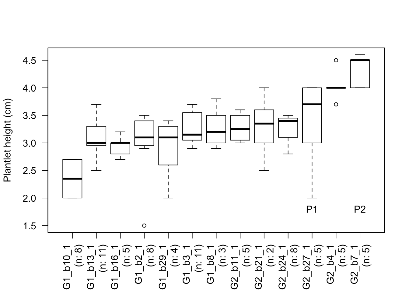
Figure 6.2: Boxplot showing plantlets heights after five weeks of culture for individuals belonging to the blue rooting cluster of diploid Artemisia tridentata subsp. tridentata. The n indicates the number of plantlets cultured for each individual. The top three performers as identified by the rooting experiment are also displayed (P1, P2).

6.4.2 R code

###~~~
#Subset to only include from blue rooting cluster
###~~~
blueHeight <- subset(subSurvHeigh, subSurvHeigh$Cluster == 'blue')

#Individual
seedID <- table(as.vector(blueHeight$SeedID))

# Create a vector named "new_order" containing the desired order to display individuals (smaller to taller)
new_order <- with(blueHeight, reorder(as.vector(blueHeight$SeedID), as.numeric(blueHeight$X5_w_height), median , na.rm=T))

###~~~
# Draw boxplot
###~~~
boxplot(as.numeric(blueHeight$X5_w_height) ~ new_order, names = paste(names(seedID), paste0("(n: ", as.vector(seedID), ")"), sep = "\n"), las=2, xlab = "", ylab = "Plantlet height (cm)", cex = .8)

#Add P1, P2
top <- which(names(seedID) %in% c("G2_b27_1", "G2_b7_1"))
text(x=top, y=1.8, c("P1", "P2"))

7 References

Lenth, Russell. 2020. Emmeans: Estimated Marginal Means, Aka Least-Squares Means. https://github.com/rvlenth/emmeans.

8 Appendix 1

Citations of all R packages used to generate this report.

[1] J. Allaire, Y. Xie, J. McPherson, et al. rmarkdown: Dynamic Documents for R. R package version 2.6. 2020. <URL: https://github.com/rstudio/rmarkdown>.

[2] C. Boettiger. knitcitations: Citations for Knitr Markdown Files. R package version 1.0.10. 2019. <URL: https://github.com/cboettig/knitcitations>.

[3] D. Ebbert. chisq.posthoc.test: A Post Hoc Analysis for Pearson’s Chi-Squared Test for Count Data. R package version 0.1.2. 2019. <URL: http://chisq-posthoc-test.ebbert.nrw/>.

[4] T. Hothorn, A. Zeileis, R. W. Farebrother, et al. lmtest: Testing Linear Regression Models. R package version 0.9-38. 2020. <URL: https://CRAN.R-project.org/package=lmtest>.

[5] S. Jackman, A. Tahk, A. Zeileis, et al. pscl: Political Science Computational Laboratory. R package version 1.5.5. 2020. <URL: http://github.com/atahk/pscl>.

[6] A. Kassambara. ggpubr: ggplot2 Based Publication Ready Plots. R package version 0.4.0. 2020. <URL: https://rpkgs.datanovia.com/ggpubr/>.

[7] R. Lenth. emmeans: Estimated Marginal Means, aka Least-Squares Means. R package version 1.5.2-1. 2020. <URL: https://github.com/rvlenth/emmeans>.

[8] R. Lenth. lsmeans: Least-Squares Means. R package version 2.30-0. 2018. <URL: https://CRAN.R-project.org/package=lsmeans>.

[9] R. V. Lenth. “Least-Squares Means: The R Package lsmeans.” In: Journal of Statistical Software 69.1 (2016), pp. 1-33. DOI: 10.18637/jss.v069.i01.

[10] E. Neuwirth. RColorBrewer: ColorBrewer Palettes. R package version 1.1-2. 2014. <URL: https://CRAN.R-project.org/package=RColorBrewer>.

[11] E. Paradis, S. Blomberg, B. Bolker, et al. ape: Analyses of Phylogenetics and Evolution. R package version 5.4-1. 2020. <URL: http://ape-package.ird.fr/>.

[12] E. Paradis and K. Schliep. “ape 5.0: an environment for modern phylogenetics and evolutionary analyses in R.” In: Bioinformatics 35 (2019), pp. 526-528.

[13] R Core Team. R: A Language and Environment for Statistical Computing. R Foundation for Statistical Computing. Vienna, Austria, 2019. <URL: https://www.R-project.org/>.

[14] B. Ripley. MASS: Support Functions and Datasets for Venables and Ripley’s MASS. R package version 7.3-53. 2020. <URL: http://www.stats.ox.ac.uk/pub/MASS4/>.

[15] M. R. Smith. TreeTools: Create, Modify and Analyse Phylogenetic Trees. R package version 1.4.0. 2020. <URL: https://CRAN.R-project.org/package=TreeTools>.

[16] W. N. Venables and B. D. Ripley. Modern Applied Statistics with S. Fourth. ISBN 0-387-95457-0. New York: Springer, 2002. <URL: http://www.stats.ox.ac.uk/pub/MASS4/>.

[17] G. R. Warnes, B. Bolker, L. Bonebakker, et al. gplots: Various R Programming Tools for Plotting Data. R package version 3.1.0. 2020. <URL: https://github.com/talgalili/gplots>.

[18] H. Wickham. forcats: Tools for Working with Categorical Variables (Factors). R package version 0.5.0. 2020. <URL: https://CRAN.R-project.org/package=forcats>.

[19] H. Wickham. ggplot2: Elegant Graphics for Data Analysis. Springer-Verlag New York, 2016. ISBN: 978-3-319-24277-4. <URL: https://ggplot2.tidyverse.org>.

[20] H. Wickham. stringr: Simple, Consistent Wrappers for Common String Operations. R package version 1.4.0. 2019. <URL: https://CRAN.R-project.org/package=stringr>.

[21] H. Wickham and J. Bryan. usethis: Automate Package and Project Setup. R package version 2.0.0. 2020. <URL: https://CRAN.R-project.org/package=usethis>.

[22] H. Wickham, W. Chang, L. Henry, et al. ggplot2: Create Elegant Data Visualisations Using the Grammar of Graphics. R package version 3.3.3. 2020. <URL: https://CRAN.R-project.org/package=ggplot2>.

[23] H. Wickham, J. Hester, and W. Chang. devtools: Tools to Make Developing R Packages Easier. R package version 2.3.2. 2020. <URL: https://CRAN.R-project.org/package=devtools>.

[24] C. O. Wilke. ggridges: Ridgeline Plots in ggplot2. R package version 0.5.2. 2020. <URL: https://wilkelab.org/ggridges>.

[25] Y. Xie. bookdown: Authoring Books and Technical Documents with R Markdown. ISBN 978-1138700109. Boca Raton, Florida: Chapman and Hall/CRC, 2016. <URL: https://github.com/rstudio/bookdown>.

[26] Y. Xie. bookdown: Authoring Books and Technical Documents with R Markdown. R package version 0.21. 2020. <URL: https://github.com/rstudio/bookdown>.

[27] Y. Xie. Dynamic Documents with R and knitr. 2nd. ISBN 978-1498716963. Boca Raton, Florida: Chapman and Hall/CRC, 2015. <URL: https://yihui.org/knitr/>.

[28] Y. Xie. formatR: Format R Code Automatically. R package version 1.7. 2019. <URL: https://github.com/yihui/formatR>.

[29] Y. Xie. “knitr: A Comprehensive Tool for Reproducible Research in R.” In: Implementing Reproducible Computational Research. Ed. by V. Stodden, F. Leisch and R. D. Peng. ISBN 978-1466561595. Chapman and Hall/CRC, 2014. <URL: http://www.crcpress.com/product/isbn/9781466561595>.

[30] Y. Xie. knitr: A General-Purpose Package for Dynamic Report Generation in R. R package version 1.30. 2020. <URL: https://yihui.org/knitr/>.

[31] Y. Xie, J. Allaire, and G. Grolemund. R Markdown: The Definitive Guide. ISBN 9781138359338. Boca Raton, Florida: Chapman and Hall/CRC, 2018. <URL: https://bookdown.org/yihui/rmarkdown>.

[32] Y. Xie, J. Cheng, and X. Tan. DT: A Wrapper of the JavaScript Library DataTables. R package version 0.16. 2020. <URL: https://github.com/rstudio/DT>.

[33] Y. Xie, C. Dervieux, and E. Riederer. R Markdown Cookbook. ISBN 9780367563837. Boca Raton, Florida: Chapman and Hall/CRC, 2020. <URL: https://bookdown.org/yihui/rmarkdown-cookbook>.

[34] G. Yu and T. T. Lam. ggtree: an R package for visualization of tree and annotation data. R package version 2.0.4. 2020. <URL: https://yulab-smu.github.io/treedata-book/>.

[35] G. Yu, T. T. Lam, H. Zhu, et al. “Two methods for mapping and visualizing associated data on phylogeny using ggtree.” In: Molecular Biology and Evolution 35 (2 2018), pp. 3041-3043. DOI: 10.1093/molbev/msy194. <URL: https://doi.org/10.1093/molbev/msy194>.

[36] G. Yu, D. Smith, H. Zhu, et al. “ggtree: an R package for visualization and annotation of phylogenetic trees with their covariates and other associated data.” In: Methods in Ecology and Evolution 8 (1 2017), pp. 28-36. DOI: 10.1111/2041-210X.12628. <URL: http://onlinelibrary.wiley.com/doi/10.1111/2041-210X.12628/abstract>.

[37] A. Zeileis and G. Grothendieck. “zoo: S3 Infrastructure for Regular and Irregular Time Series.” In: Journal of Statistical Software 14.6 (2005), pp. 1-27. DOI: 10.18637/jss.v014.i06.

[38] A. Zeileis, G. Grothendieck, and J. A. Ryan. zoo: S3 Infrastructure for Regular and Irregular Time Series (Z’s Ordered Observations). R package version 1.8-8. 2020. <URL: http://zoo.R-Forge.R-project.org/>.

[39] A. Zeileis and T. Hothorn. “Diagnostic Checking in Regression Relationships.” In: R News 2.3 (2002), pp. 7-10. <URL: https://CRAN.R-project.org/doc/Rnews/>.

[40] A. Zeileis, C. Kleiber, and S. Jackman. “Regression Models for Count Data in R.” In: Journal of Statistical Software 27.8 (2008). <URL: http://www.jstatsoft.org/v27/i08/>.

9 Appendix 2

Version information about R, the operating system (OS) and attached or R loaded packages. This appendix was generated using sessionInfo().

## R version 3.6.1 (2019-07-05)
## Platform: x86_64-apple-darwin15.6.0 (64-bit)
## Running under: macOS Mojave 10.14.6
## 
## Matrix products: default
## BLAS:   /Library/Frameworks/R.framework/Versions/3.6/Resources/lib/libRblas.0.dylib
## LAPACK: /Library/Frameworks/R.framework/Versions/3.6/Resources/lib/libRlapack.dylib
## 
## locale:
## [1] en_US.UTF-8/en_US.UTF-8/en_US.UTF-8/C/en_US.UTF-8/en_US.UTF-8
## 
## attached base packages:
## [1] stats     graphics  grDevices utils     datasets  methods   base     
## 
## other attached packages:
##  [1] moments_0.14             forcats_0.5.0            TreeTools_1.4.0         
##  [4] ggridges_0.5.2           stringr_1.4.0            ape_5.4-1               
##  [7] ggtree_2.0.4             ggpubr_0.4.0             ggplot2_3.3.2           
## [10] chisq.posthoc.test_0.1.2 DT_0.16                  lsmeans_2.30-0          
## [13] emmeans_1.5.2-1          lmtest_0.9-38            zoo_1.8-8               
## [16] pscl_1.5.5               RColorBrewer_1.1-2       gplots_3.1.0            
## [19] devtools_2.3.2           usethis_1.6.3            formatR_1.7             
## [22] knitcitations_1.0.10     bookdown_0.21            rmarkdown_2.4           
## [25] knitr_1.30              
## 
## loaded via a namespace (and not attached):
##   [1] colorspace_1.4-1    ggsignif_0.6.0      ellipsis_0.3.1     
##   [4] rio_0.5.16          rprojroot_1.3-2     estimability_1.3   
##   [7] fs_1.5.0            farver_2.0.3        remotes_2.2.0      
##  [10] bit64_4.0.5         fansi_0.4.1         mvtnorm_1.1-1      
##  [13] lubridate_1.7.9     RefManageR_1.2.12   xml2_1.3.2         
##  [16] codetools_0.2-16    R.methodsS3_1.8.1   pkgload_1.1.0      
##  [19] jsonlite_1.7.1      broom_0.7.1         R.oo_1.24.0        
##  [22] BiocManager_1.30.10 compiler_3.6.1      httr_1.4.2         
##  [25] rvcheck_0.1.8       backports_1.1.10    Matrix_1.2-18      
##  [28] assertthat_0.2.1    lazyeval_0.2.2      cli_2.1.0          
##  [31] htmltools_0.5.0     prettyunits_1.1.1   tools_3.6.1        
##  [34] igraph_1.2.6        coda_0.19-4         gtable_0.3.0       
##  [37] glue_1.4.2          dplyr_1.0.2         fastmatch_1.1-0    
##  [40] Rcpp_1.0.5          carData_3.0-4       cellranger_1.1.0   
##  [43] vctrs_0.3.4         nlme_3.1-149        gbRd_0.4-11        
##  [46] xfun_0.18           rbibutils_1.4       ps_1.4.0           
##  [49] openxlsx_4.2.2      testthat_2.3.2      lifecycle_0.2.0    
##  [52] phangorn_2.5.5      gtools_3.8.2        rstatix_0.6.0      
##  [55] MASS_7.3-53         scales_1.1.1        hms_0.5.3          
##  [58] parallel_3.6.1      yaml_2.2.1          curl_4.3           
##  [61] memoise_1.1.0       stringi_1.5.3       highr_0.8          
##  [64] desc_1.2.0          tidytree_0.3.3      caTools_1.18.0     
##  [67] pkgbuild_1.1.0      zip_2.1.1           bibtex_0.4.2.3     
##  [70] Rdpack_2.1          rlang_0.4.8         pkgconfig_2.0.3    
##  [73] bitops_1.0-6        evaluate_0.14       lattice_0.20-41    
##  [76] purrr_0.3.4         labeling_0.3        treeio_1.10.0      
##  [79] htmlwidgets_1.5.2   cowplot_1.1.0       bit_4.0.4          
##  [82] processx_3.4.4      tidyselect_1.1.0    plyr_1.8.6         
##  [85] magrittr_1.5        R6_2.4.1            generics_0.0.2     
##  [88] pillar_1.4.6        haven_2.3.1         foreign_0.8-75     
##  [91] withr_2.3.0         abind_1.4-5         tibble_3.0.4       
##  [94] crayon_1.3.4        car_3.0-10          KernSmooth_2.23-17 
##  [97] grid_3.6.1          readxl_1.3.1        data.table_1.12.8  
## [100] callr_3.5.1         digest_0.6.25       R.cache_0.14.0     
## [103] xtable_1.8-4        tidyr_1.1.2         R.utils_2.10.1     
## [106] munsell_0.5.0       quadprog_1.5-8      sessioninfo_1.1.1

10 Appendix 3

Tissue culture data at the basis of analyses presented in step 3.

11 Appendix 4

In vitro survival and growth data for plantlets at the basis of analyses presented in step 4.